7. Sorting & Searching
🔀 Comparison and linear sorts, binary search, and binary search on the answer.
The unifying idea. Every algorithm here exploits order: either it creates order (sorting) or it assumes order exists and queries it cheaply (searching). The loop invariant is the tool that makes every loop here correct.
A. Loop invariants — the loop-correctness tool
Why · know a loop is right without tracing it. Where · every loop on this sheet; binary search is the canonical case where getting it wrong causes off-by-ones or infinite loops.
An invariant is a claim about your variables that stays true on every iteration. Prove it holds at the start, each step preserves it, and at termination it gives the result — no tracing required.
Example problem: find the maximum value in a = [3, 1, 4, 1, 5].
Invariant: best holds the maximum of all elements seen so far.
a = [3, 1, 4, 1, 5]
best = a[0]           # invariant: best = max(a[0..i])
for x in a[1:]:
    if x > best:
        best = x
# best = 5
Figure 1 · Loop invariant: find-max trace.
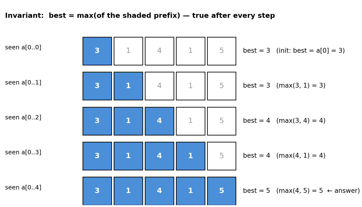
best always holds the max of the prefix seen so far. The invariant holds before the loop,
after each step, and at termination — so the result is correct by construction.
The three checks:
- Start: invariant holds before the first iteration.
- Maintenance: each step preserves the invariant.
- Termination: invariant + exit condition gives the answer.
The same three checks apply to every loop on this sheet — Section B is the canonical case.
B. Binary search
Why · \(O(\log n)\) find in a sorted array — each step eliminates half the remaining range. Where · any sorted collection; the foundation of Section C’s “binary search on the answer.”
Example problem: find the index of target in sorted nums, or -1 if absent.
Invariant: if the target is present, it lies within nums[left..right]. Every step halves the range while preserving this — off-by-one errors are exactly the bugs that break it.
Algorithm:
nums = [1, 4, 7, 9, 15]
target = 9

left, right = 0, len(nums) - 1   # invariant: if target present, it's in nums[left..right]
while left <= right:
    mid = (left + right) // 2
    if nums[mid] == target:
        result = mid
        break
    elif nums[mid] < target:
        left = mid + 1             # target can't be in [left..mid] — eliminate left half
    else:
        right = mid - 1            # target can't be in [mid..right] — eliminate right half
# result: 3
Figure 2 · Binary search halving: [1,4,7,9,15], target = 9.
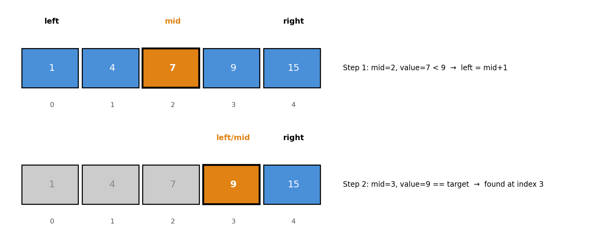
Each row is one step. Orange = mid element. Grey = eliminated range. Two steps reach index 3.
Mechanism trace:
-
left=0, right=4,mid=2, value=7. 9 > 7 →left = 3. -
left=3, right=4,mid=3, value=9. Match → found at index 3.
Cost: \(O(\log n)\) — each step halves the remaining range, so after \(k\) steps at most \(\lceil n / 2^k \rceil\) elements remain. The range hits 1 when \(2^k = n\), i.e. \(k = \lceil \log_2 n \rceil\) steps.
Python: bisect.bisect_left(nums, target) for the standard library version.
C. Binary search on the answer
Why · turn “find the minimum \(X\) satisfying a condition” into \(O(\log(\text{range}))\) by binary-searching the answer space instead of the array. Where · capacity/speed/threshold problems where “is \(X\) feasible?” is computable in \(O(n)\).
Invariant: if a valid answer exists, it lies within [left, right] — identical to binary search on an array, but the “array” is the answer space.
The pattern: if a yes/no feasibility question is monotone — once the answer is “yes” for some \(X\), it stays “yes” for all larger \(X\) — binary-search the answer space.
Example problem: given banana piles [3, 6, 7, 11] and hours = 8, find the minimum integer speed (bananas/hour) such that all piles are eaten in time. Each pile takes ⌈pile / speed⌉ hours — you can’t split an hour across piles.
Search range [1, max(piles)]: speed 0 is undefined; at max(piles) every pile takes 1 hour so total = len(piles) ≤ hours — a valid answer always exists. Feasibility is monotone (faster is always at least as good), so binary search on this range finds the minimum valid speed.
Figure 3 · Answer space [1..11]: feasibility above, shrinking search window below.
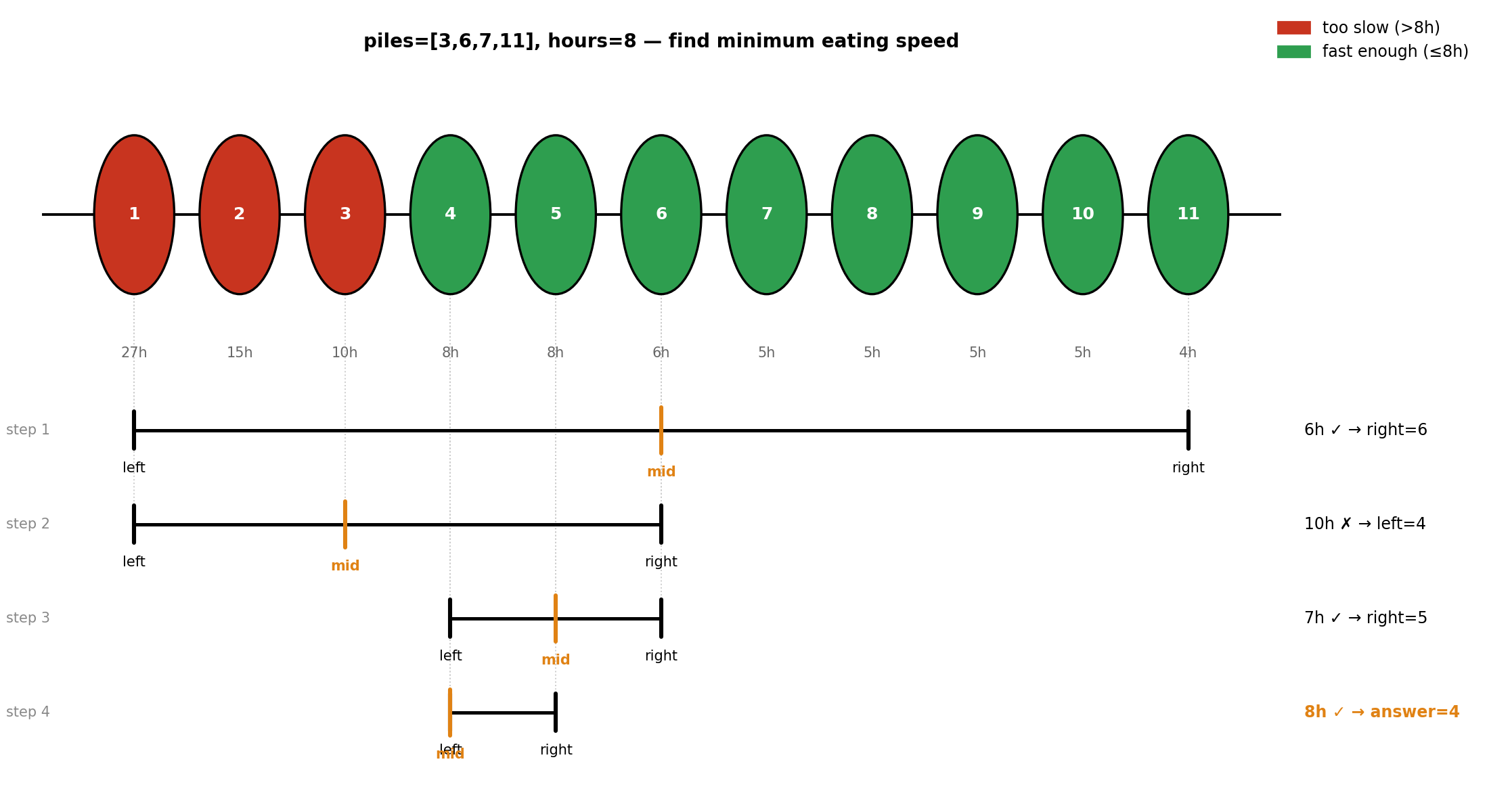
Top: each circle is one candidate speed; the label shows hours needed. Red = too slow, green = fast enough. The all-red-then-all-green boundary is what makes binary search valid. Bottom: each row is one step — the grey window spans [left, right], the orange tick marks mid, and the window shrinks until only the answer remains.
Algorithm:
piles = [3, 6, 7, 11]
hours = 8

def can_finish(speed):
    return sum((pile + speed - 1) // speed for pile in piles) <= hours

left, right = 1, max(piles)
while left < right:
    mid = (left + right) // 2
    if can_finish(mid):
        right = mid
    else:
        left = mid + 1
# left is the minimum valid speed: 4
Mechanism trace:
-
left=1, right=11,mid=6.can_finish(6)= 1+1+2+2 = 6 ≤ 8 →right=6. -
left=1, right=6,mid=3.can_finish(3)= 1+2+3+4 = 10 > 8 →left=4. -
left=4, right=6,mid=5.can_finish(5)= 1+2+2+3 = 8 ≤ 8 →right=5. -
left=4, right=5,mid=4.can_finish(4)= 1+2+2+3 = 8 ≤ 8 →right=4. -
left=4, right=4. Answer = 4.
Cost: \(O(n \log(\max(\text{piles})))\) — binary search on the range, feasibility check costs \(O(n)\).
Recognition trigger: “minimum/maximum \(X\) such that \(P(X)\) holds” where \(P\) is monotone → binary search on the answer. See the upcoming pattern-triggers post for the trigger row.
D. Comparison sorts
Why · \(O(n \log n)\) is the best possible for comparison-based sorting — any algorithm that only compares elements needs at least \(\Omega(n \log n)\) comparisons in the worst case. Where · whenever you need sorted order and key type supports comparison.
Figure 4 · O(n²) vs O(n log n) — where the crossover happens.
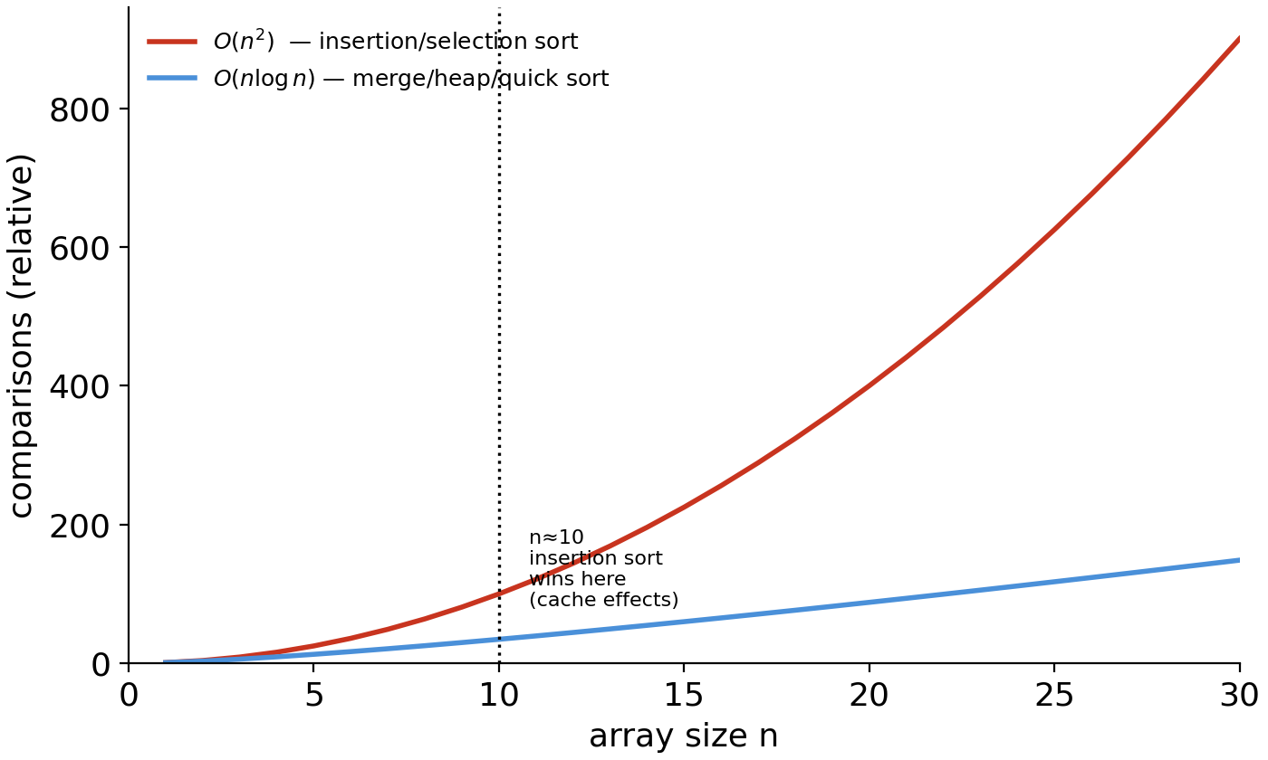
Above n≈10, O(n log n) wins decisively. Below n≈10, insertion sort’s cache-friendly access beats merge sort in practice despite worse asymptotic behaviour.
Running example: [5, 3, 8, 1, 4] for merge sort and quicksort traces.
Merge sort (recursive — see Recursion & Backtracking for the recursion tree): Repeatedly halve the array until each piece has one element (trivially sorted), then merge adjacent sorted pairs back up. Merging two sorted arrays is linear — scan both from the left, always taking the smaller element. The recursion tree has depth \(\log n\), each level doing \(O(n)\) merge work total.
Invariant: after merge, the output array contains the same elements as both halves, in sorted order.
def merge_sort(array):
    if len(array) <= 1:
        return array
    mid = len(array) // 2
    left_half  = merge_sort(array[:mid])
    right_half = merge_sort(array[mid:])
    return merge(left_half, right_half)

def merge(left, right):
    result = []
    while left and right:
        if left[0] <= right[0]:
            result.append(left.pop(0))    # stable: equal elements keep original order
        else:
            result.append(right.pop(0))
    return result + left + right
Trace on [5,3,8,1,4]: split → [5,3] and [8,1,4] → recurse → merge [3,5] with [1,4,8] → [1,3,4,5,8].
Heap sort (uses the heap from Hierarchical Structures): Two phases: first build a min-heap from the array in \(O(n)\); then repeatedly extract the minimum in \(O(\log n)\). The extractions come out in sorted order. No recursion — all work is heap bookkeeping on a flat array.
import heapq

def heap_sort(array):
    heap = array[:]
    heapq.heapify(heap)                   # O(n) build
    return [heapq.heappop(heap) for _ in heap[:]]   # n × O(log n) pops
Trace on [5,3,8,1,4]: heapify → [1,3,8,5,4]. Pops in order: 1, 3, 4, 5, 8 → result [1,3,4,5,8]. (See Hierarchical Structures Section B for the sift-down mechanics.)
Build-heap is \(O(n)\); \(n\) pops cost \(O(n \log n)\) total. In-place variant exists but heapq is cleaner.
Quicksort (recursive — average \(O(n \log n)\), worst \(O(n^2)\) on sorted input): Pick a pivot element, partition the array into three groups — elements smaller than the pivot, equal, and larger — then recurse on the smaller and larger groups. The pivot is in its final sorted position after each partition. Average depth is \(O(\log n)\) with a random pivot; worst case \(O(n)\) depth if the pivot is always the min or max.
Invariant: after partitioning, every element in left is < pivot and every element in right is > pivot — the pivot is in its final position.
def quicksort(array):
    if len(array) <= 1:
        return array
    pivot = array[len(array) // 2]
    left   = [x for x in array if x < pivot]
    middle = [x for x in array if x == pivot]
    right  = [x for x in array if x > pivot]
    return quicksort(left) + middle + quicksort(right)
Trace on [5,3,8,1,4], pivot=8: left=[5,3,1,4], middle=, right=[] → recurse left.
Cost summary:
| Sort | Time | Space | Stable | Use when |
|---|---|---|---|---|
| Merge | \(O(n \log n)\) | \(O(n)\) | Yes | Need stable sort |
| Heap | \(O(n \log n)\) | \(O(1)\) | No | In-place required |
| Quick | \(O(n \log n)\) avg | \(O(\log n)\) | No | Fastest in practice |
In practice: use sorted() or list.sort() — Python’s Timsort (hybrid merge + insertion sort, stable, \(O(n \log n)\)) is faster than any manual implementation.
E. Linear sorts
Why · break the \(\Omega(n \log n)\) comparison lower bound by exploiting key structure — \(O(n+k)\) when the key range \(k\) is small. Where · integer keys with bounded range (scores, small IDs); fixed-width strings or integers.
These algorithms don’t compare elements to each other. Instead they use the value itself as an index or bucket address — so the sorted position of an element is computed directly from its value, not derived from comparisons with other elements.
Figure 5 · Counting sort: count → start positions → output.
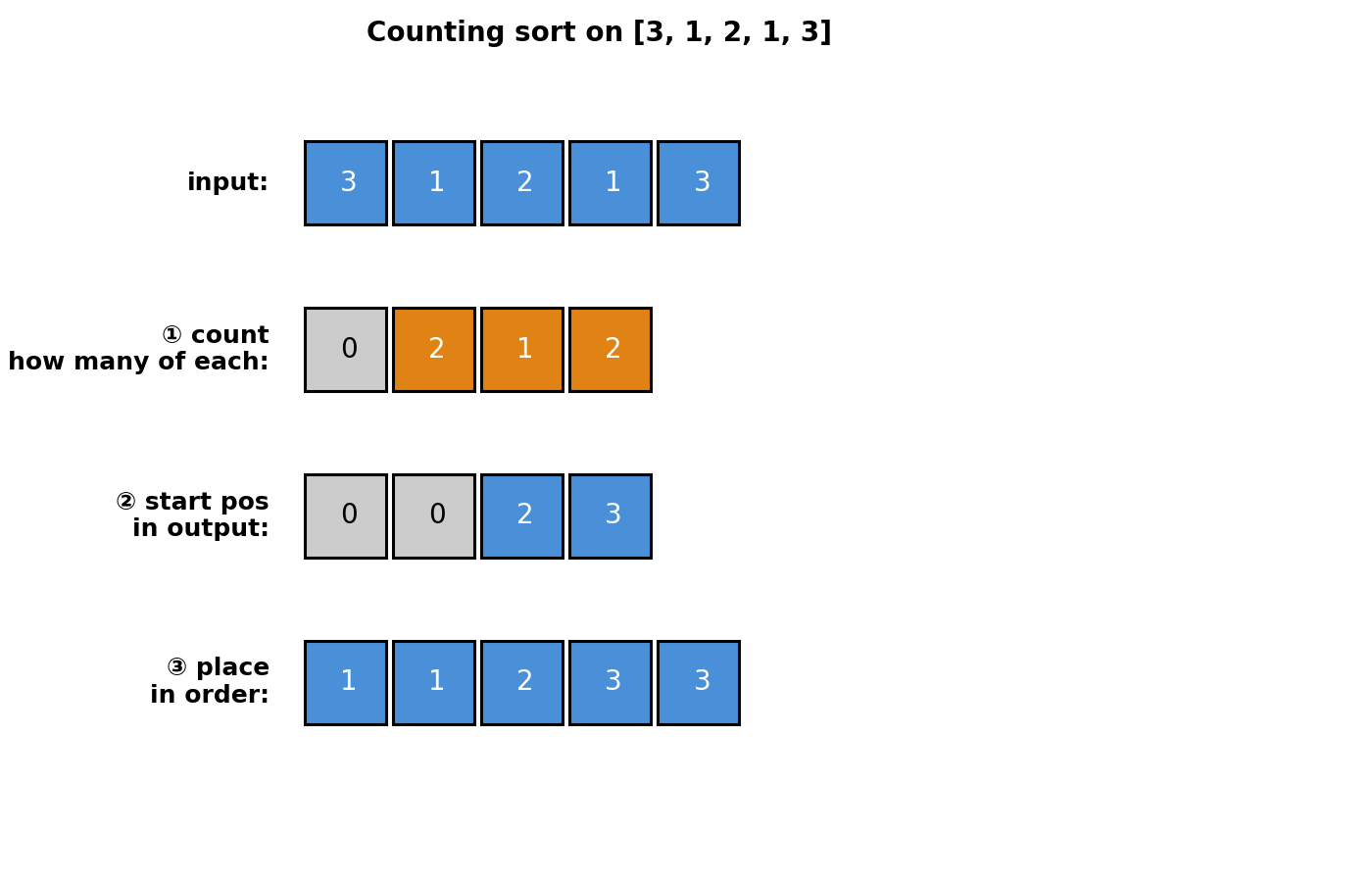
Three steps on [3,1,2,1,3]: ① count how many of each value appear; ② convert counts to start positions (where each value’s run begins in the output); ③ place each element at its start position.
Counting sort — keys are integers in \([0, k)\):
data = [3, 1, 2, 1, 3]
k = 4                              # keys are 0, 1, 2, 3

counts = [0] * k
for x in data:
    counts[x] += 1                 # count occurrences

output = []
for value, count in enumerate(counts):
    output.extend([value] * count) # place in order
# output: [1, 1, 2, 3, 3]
Cost: \(O(n + k)\) — one pass over the data to fill counts (\(n\)), one pass over the range to emit output (\(k\)). When \(k = O(n)\), this is \(O(n)\).
Figure 6 · Radix sort: two stable passes by digit.
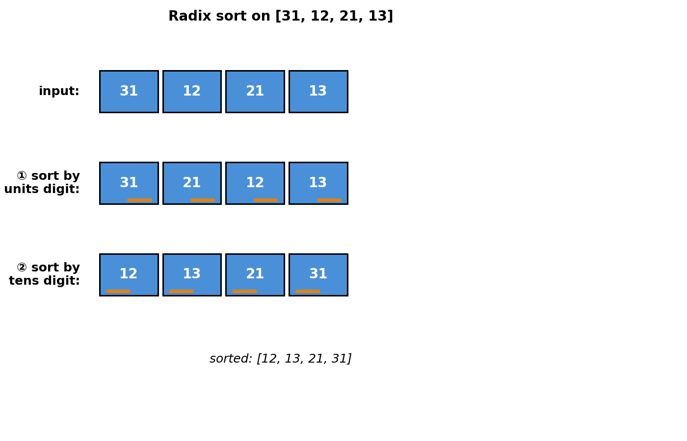
Each pass applies counting sort to one digit (underlined in orange). Sorting least-significant first preserves earlier-digit order across passes — stability is what makes this work.
Radix sort — sort \(d\)-digit numbers digit by digit (least-significant first) using counting sort as the stable inner sort:
def radix_sort(nums, base=10):
    max_digits = len(str(max(nums)))
    for digit in range(max_digits):       # least-significant digit first
        buckets = [[] for _ in range(base)]
        for n in nums:
            buckets[(n // base**digit) % base].append(n)  # shift right by digit positions, take last digit
        nums = [n for bucket in buckets for n in bucket]
    return nums
Trace on [170, 45, 75, 90]: sort by units → [170,90,45,75]; sort by tens → [45,75,90,170]. Each pass is stable, so earlier-digit order is preserved.
Cost: \(O(d \cdot (n + k))\) — \(d\) passes, each a full counting sort costing \(O(n + k)\). For fixed-width integers \(d\) is constant, giving \(O(n)\).
🔗 Connections
- Loop invariant concept introduced here: Foundations has the general definition.
- Merge/quicksort build on recursion model: Recursion & Backtracking.
- Heapsort builds on the heap: Hierarchical Structures.
- Sorting used in merge intervals and Kruskal’s MST: Array & String Techniques, Graphs.
- Binary-search-on-answer trigger in the pattern sheet: the upcoming pattern-triggers post.