6. Recursion & Backtracking
🔁 The recursion mental model and the choose/explore/un-choose backtracking template.
The unifying idea. Recursion reduces a problem to a smaller version of itself, hitting a base case to stop. Backtracking is recursion over a choice tree: at each node you pick one option, recurse into it, then undo the pick before trying the next. The template is the same every time; only the base case and the choice set change.
A. Recursion mental model
Why · express solutions that naturally decompose into smaller versions of the same problem. Where · any algorithm that halves or shrinks its input: merge sort, binary search, tree traversal (Graphs).
Every recursive function needs exactly two things: a base case that stops the recursion, and a recursive case that makes the input strictly smaller. If both hold, the function is correct by induction. You never need to trace the full call chain manually.
Example problem: compute \(n!\) (factorial).
Algorithm:
def factorial(n):
    if n == 0:               # base case: stop here
        return 1
    return n * factorial(n - 1)   # recursive case: shrink n by 1

factorial(4)   # → 24
Figure 1 · Recursion call stack for factorial(4).
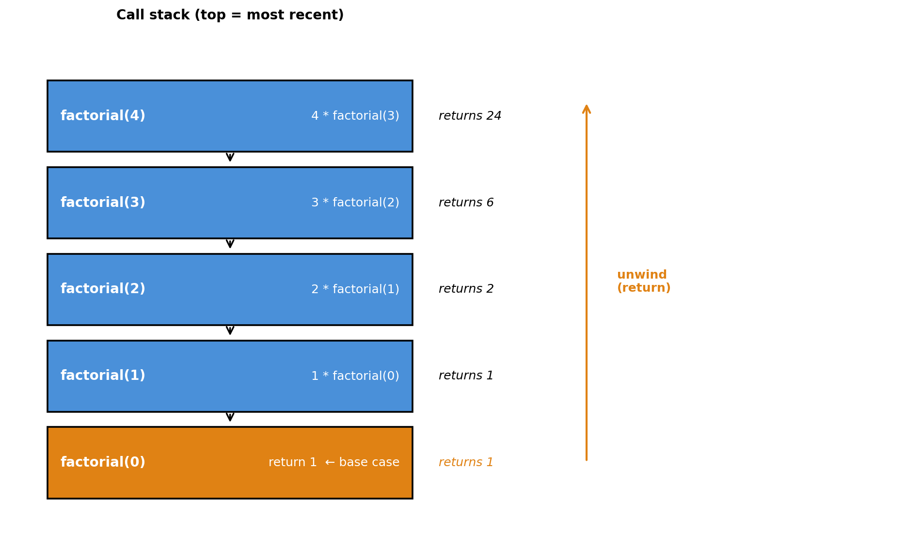
Each frame makes one smaller call until n=0 (orange, base case). The results unwind upward: 1 → 1 → 2 → 6 → 24.
Mechanism trace — factorial(3):
-
factorial(3): 3 ≠ 0 → callfactorial(2). -
factorial(2): 2 ≠ 0 → callfactorial(1). -
factorial(1): 1 ≠ 0 → callfactorial(0). -
factorial(0): base case → return 1. - Unwind: \(1 \cdot 1 = 1\) → \(2 \cdot 1 = 2\) → \(3 \cdot 2 = 6\).
Cost: \(O(n)\) calls, \(O(n)\) stack space — one frame pushed per recursive call, up to depth \(n\).
Add memoization here → that’s Dynamic Programming, deliberately deferred from this atlas.
[DP expansion — ~4 lines] When subproblems repeat (e.g.
fib(3)called multiple times), plain recursion recomputes them. Add a cache:memo = {}; if n in memo: return memo[n]. This is memoization — the top-down form of DP. The call tree becomes a DAG; cost drops from \(O(2^n)\) to \(O(n)\). Bottom-up DP builds the same table iteratively without the call stack overhead.
B. Backtracking template and subsets application
Why · explore every combination of choices without writing nested loops of unknown depth. Where · subsets, permutations, combinations, constraint satisfaction — all are instances of this one template.
Backtracking is DFS over a choice tree (see Graphs for DFS). At each node: choose one option, explore its subtree, unchoose to restore state, then try the next option.
The template (only the base case and choices differ across problems):
results = []

def backtrack(path, choices):
    if base_case(path):           # a complete answer — record it
        results.append(path[:])
        return
    for choice in choices:
        path.append(choice)                         # choose
        backtrack(path, remaining(choices, choice)) # explore
        path.pop()                                  # unchoose
Subsets application
Why · generate all \(2^n\) subsets of a set — the canonical backtracking instance. Where · power sets, feature combinations, any “include or exclude each item” problem.
How subsets differs from the template:
- No base case guard — record unconditionally at every node, because every path is a valid subset.
-
remaining(choices, choice)= elements after the current index (i + 1) — avoids duplicates.
nums = [1, 2, 3]
results = []

def subsets(start, path):
    results.append(path[:])          # every path is a valid subset
    for i in range(start, len(nums)):
        path.append(nums[i])         # choose nums[i]
        subsets(i + 1, path)         # explore: only later elements
        path.pop()                   # unchoose

subsets(0, [])
# results: [[], [1], [1,2], [1,2,3], [1,3], [2], [2,3], [3]]
Figure 2 · Choice tree for subsets of [1, 2, 3].
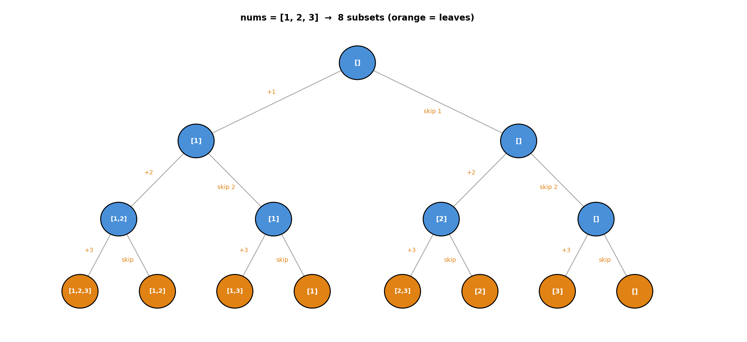
Each edge is a choice (+1 = include, skip = exclude). Every path from root to leaf is one subset. Orange leaves are the 8 results — the empty set is the root itself.
Mechanism trace (first branch of Figure 2):
-
subsets(0, []): record[]. Choose 1 → path. -
subsets(1, [1]): record. Choose 2 → path[1,2]. -
subsets(2, [1,2]): record[1,2]. Choose 3 → path[1,2,3]. -
subsets(3, [1,2,3]): record[1,2,3]. No choices left → return. - Unchoose 3 →
[1,2]. Unchoose 2 →. Choose 3 → path[1,3]… and so on.
Cost: \(O(2^n \cdot n)\) — \(2^n\) subsets, each up to \(n\) elements to copy.
[DP expansion — ~3 lines] If you only need to count subsets satisfying a constraint (e.g. “how many subsets sum to target \(T\)?”), backtracking is \(O(2^n)\) but DP is \(O(n \cdot T)\). Subproblems overlap: “can we reach sum \(s\) using items \(0..i\)?” recurs identically from many paths. Cache the answer and the exponential collapse to polynomial.
C. Permutations
Why · generate all \(n!\) orderings of \(n\) items — every item used exactly once. Where · scheduling, anagram generation, any “arrange all items” problem.
Example problem: all permutations of nums = [1, 2, 3].
Difference from subsets: every item is used exactly once, and order matters. Track which items have
been used with a used array; recurse until the path is full.
Figure 3 · Permutation tree for [1, 2, 3].
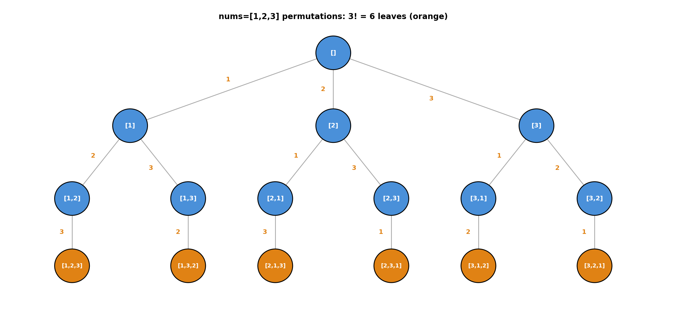
Three choices at the root (any of 1, 2, 3 can go first), two at each second level, one at the third. Six leaves — one per permutation.
Algorithm:
nums = [1, 2, 3]
results = []

def permutations(path, used):
    if len(path) == len(nums):      # all items placed — record
        results.append(path[:])
        return
    for i in range(len(nums)):
        if used[i]:
            continue                # skip already-used items
        used[i] = True
        path.append(nums[i])
        permutations(path, used)
        path.pop()
        used[i] = False

permutations([], [False] * len(nums))
# results: all 6 permutations of [1,2,3]
Mechanism trace (first permutation):
-
used=[F,F,F]. Choose index 0 (value 1) → path,used=[T,F,F]. - Choose index 1 (value 2) → path
[1,2],used=[T,T,F]. - Choose index 2 (value 3) → path
[1,2,3]. Full → record. (Figure 3.) - Unchoose 3, unchoose 2, choose index 2 (value 3) → path
[1,3]…
Cost: \(O(n! \cdot n)\) — \(n!\) permutations, each of length \(n\).
D. Combinations
Why · generate all \(\binom{n}{k}\) subsets of exactly size \(k\) — pruning makes it much faster than generating all subsets and filtering. Where · fixed-size selections, \(k\)-element feature sets, any “choose exactly \(k\)” problem.
Example problem: all combinations of size k = 2 from nums = [1, 2, 3].
Difference from subsets: only paths of exactly length k are answers. Pruning: if the remaining
elements can’t fill the path to size k, stop early.
Figure 4 · Pruning cuts branches that can’t reach k = 2.
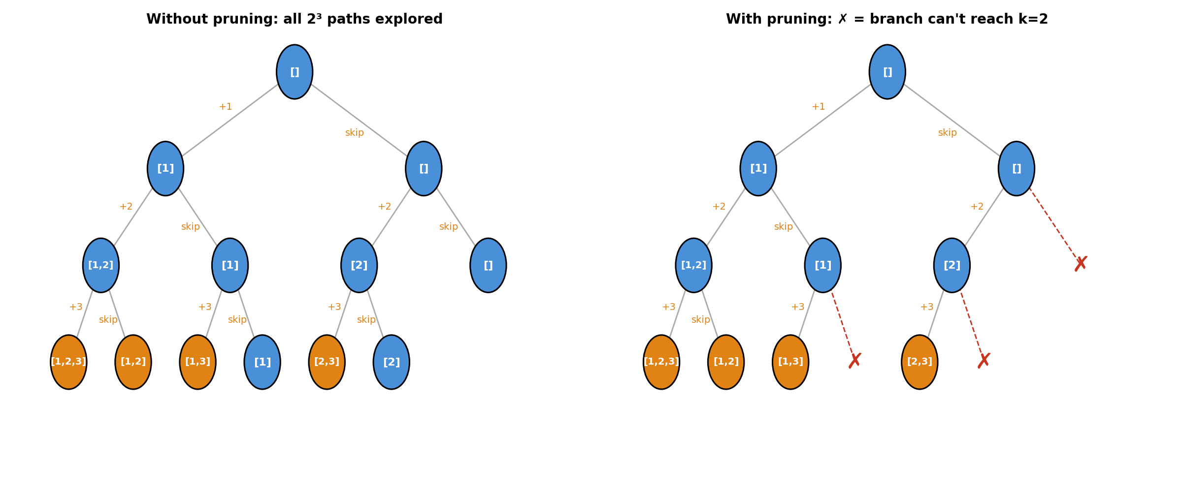
Left: all paths explored without pruning (\(2^3 = 8\) paths). Right: branches marked ✗ are cut because the remaining elements are fewer than still needed — only \(\binom{3}{2} = 3\) paths remain.
Algorithm:
nums = [1, 2, 3]
k = 2
results = []

def combinations(start, path):
    if len(path) == k:              # reached target size — record
        results.append(path[:])
        return
    remaining = len(nums) - start
    needed = k - len(path)
    if remaining < needed:          # can't reach k — prune this branch
        return
    for i in range(start, len(nums)):
        path.append(nums[i])
        combinations(i + 1, path)
        path.pop()

combinations(0, [])
# results: [[1,2], [1,3], [2,3]]
Mechanism trace:
-
start=0, path=[]. Need 2. Remaining=3. OK → choose 1 → path. -
start=1, path=[1]. Need 1. Remaining=2. OK → choose 2 → path[1,2]. Full → record. - Unchoose 2 → choose 3 → path
[1,3]. Full → record. - Unchoose 3, unchoose 1 → choose 2 → path. Need 1. Remaining=1. OK → choose 3 →
[2,3]. Record.
Cost: \(O\!\left(\binom{n}{k} \cdot k\right)\) with pruning — \(\binom{n}{k}\) valid paths, each of length \(k\) to copy. Without pruning every node in the \(2^n\) subset tree would be visited.
🔗 Connections
- Recursive cost analysis (master theorem): Foundations.
- Recursion used in merge sort and quicksort: Sorting & Searching.
- Backtracking = DFS over a choice tree: Graphs.
- Backtracking trigger in the pattern sheet: the upcoming pattern-triggers post.