5. Hierarchical Structures
🌳 Ordered and ranked access: BST and balanced trees, heaps, tries, and union-find.
These are the same two memory primitives from Linear Structures, just with a structural invariant added. Three of the four structures are pointer-chained nodes (like a linked list), but the pointers are constrained by an ordering or grouping rule. The heap is different: it is contiguous, like a dynamic array, with no pointers. Without the invariant, you would just have a linked list or a flat array.
| Structure | Memory primitive | Invariant added |
|---|---|---|
| BST (Binary Search Tree) | Pointer-chained | left child < node < right child |
| Heap | Contiguous array | parent \(\leq\) children, via index math \(i \to 2i+1,\ 2i+2\) |
| Trie (prefix tree) | Pointer-chained | each edge is one character |
| Union-Find | Pointer-chained | every pointer leads toward a root; same root = same group |
A. BST (Binary Search Tree) — ordered access via a structural invariant
Why ·
O(log n)find, insert, and delete on a dynamic set of keys. Where · any time you need to maintain a sorted order as items are inserted and deleted: sorted iteration, range queries, next/previous element in sorted order.
A BST is pointer-chained like a linked list, but each node has two pointers instead of one: left for
keys smaller than the current node, right for keys larger. At each step you compare the target key
to the current node and follow exactly one pointer. That comparison replaces an O(n) scan.
Invariant: every node’s key is greater than all keys in its left subtree and less than all keys in its right subtree. Find becomes a binary decision at each node: go left or go right.
Example problem: maintain a dynamic set of integers with fast find and insert.
Algorithm — find(node, key) and bst_insert(root, key):
def find(node, key):
    if node is None or node.key == key:
        return node
    if key < node.key:
        return find(node.left, key)    # answer must be in left subtree
    return find(node.right, key)       # answer must be in right subtree

def bst_insert(root, key):
    if root is None:
        return Node(key)               # place the new node here
    if key < root.key:
        root.left = bst_insert(root.left, key)
    elif key > root.key:
        root.right = bst_insert(root.right, key)
    return root

# Build the tree: insert 8, 3, 10, 1, 6, 9, 14 (balanced result)
root = None
for k in [8, 3, 10, 1, 6, 9, 14]:
    root = bst_insert(root, k)
Inserting keys in sorted order (e.g. 1, 3, 6, 8) always goes right at every step. No left subtrees ever form, producing the degenerate chain shown on the right of Figure 1.
Figure 1 · BST find path and the cost of imbalance.
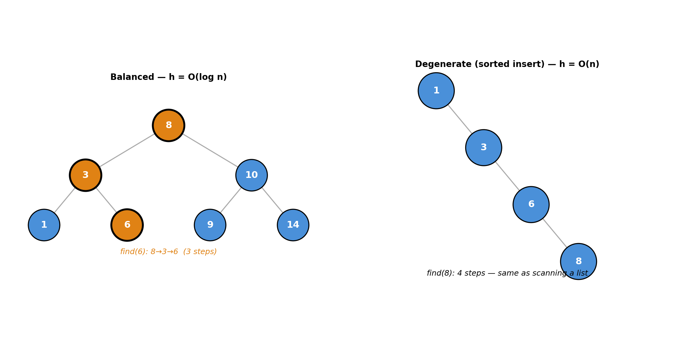
Left: balanced BST built from [8,3,10,1,6,9,14]. find(6) takes 3 steps (8→3→6), O(log n). Right: degenerate BST from inserting [1,3,6,8] in sorted order. A right-linked chain, O(n).
Mechanism trace — find(6) in the balanced BST above (root = 8):
- 6 < 8 → go left to node 3.
- 6 > 3 → go right to node 6.
- 6 == 6 → found. 3 comparisons,
O(h)whereh= tree height.
Why balancing matters: if keys arrive in sorted order, every new node becomes the rightmost child.
Height h grows to O(n). A balanced BST (AVL and red-black are two variants) restores height after
each insert via local pointer rewirings (rotations), keeping h = O(log n) guaranteed.
Python exposes no balanced BST directly. Use sortedcontainers.SortedList for O(log n) ops.
Costs: find/insert/delete O(log n) balanced · O(n) degenerate · space O(n).
B. Binary heap — ranked access via the heap property
Why ·
O(log n)push and pop,O(1)peek. The structure you reach for whenever you need to repeatedly extract the minimum (or maximum). Where · top-K problems, scheduling, Dijkstra (Graphs), heapsort (Sorting & Searching).
A heap is contiguous: a dynamic array (same primitive as Section A of Linear Structures). There are no pointers; the tree structure exists only in the index arithmetic.
Invariant: stored as a contiguous array representing a complete binary tree (every level fully filled except the last, which fills left-to-right; this shape is what makes the index math work). Every parent’s value is ≤ its children’s values (min-heap). This means the minimum is always at index 0.
Index arithmetic, for any node at index i:
- Left child: \(2i + 1\)
- Right child: \(2i + 2\)
- Parent: \((i - 1) // 2\)
Figure 2 · Heap array ↔ complete binary tree with index annotations.
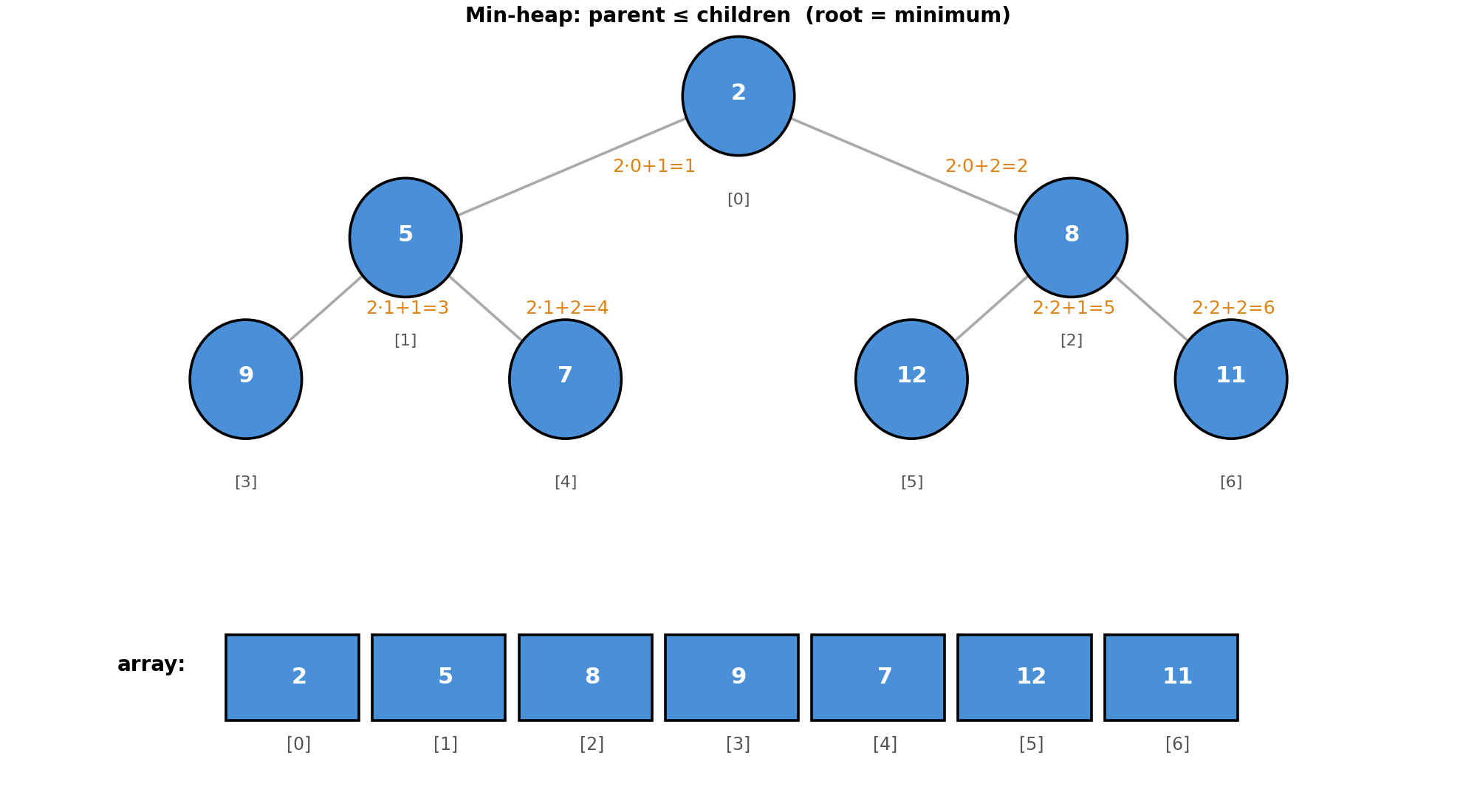
The same heap stored as an array (bottom) and drawn as a tree (top). Each edge shows the index formula; the root (index 0) is always the minimum.
Example problem: maintain a collection and repeatedly extract the smallest element.
Algorithm:
import heapq

heap = []
for value in [5, 3, 8]:
    heapq.heappush(heap, value)
# heap = [3, 5, 8], root is always the minimum

minimum = heap[0]              # O(1) peek — no removal
smallest = heapq.heappop(heap) # O(log n) — removes and returns minimum
Figure 3 · Heap push: append then bubble up to restore invariant.
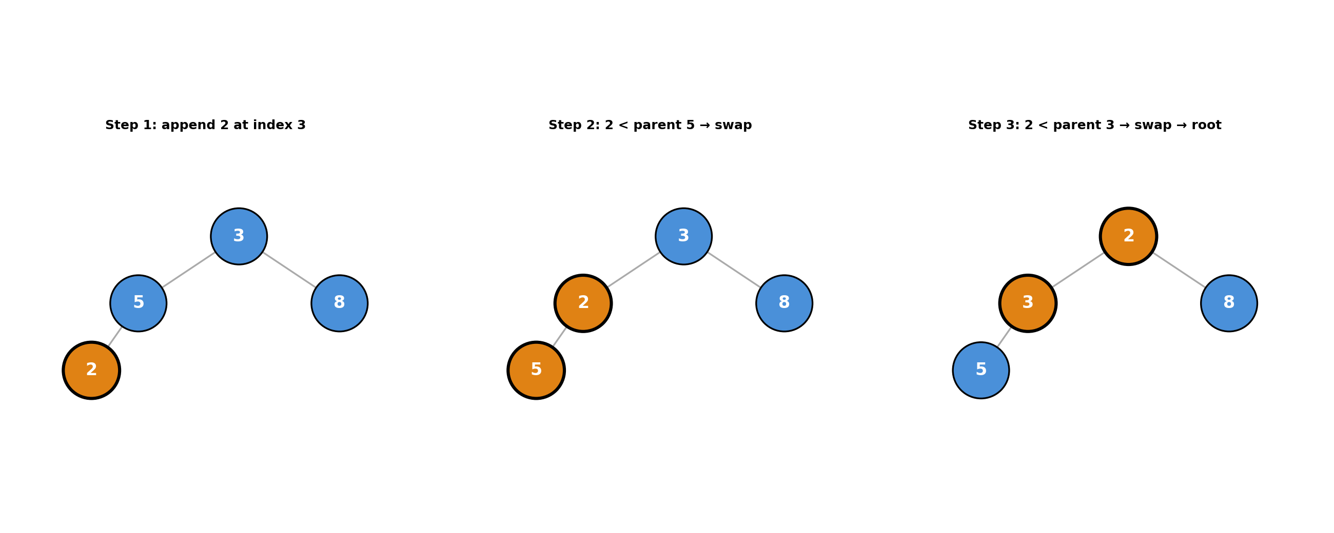
Step 1: append 2 at the end. Step 2: 2 < parent 5 → swap. Step 3: 2 < parent 3 → swap to root. Each swap restores the parent ≤ children invariant one level up.
Mechanism trace — heappush(heap, 2) on [3, 5, 8]:
- Append 2 at index 3. Heap =
[3, 5, 8, 2]. - Parent of index 3 is index 1 (value 5). 2 < 5 → swap. Heap =
[3, 2, 8, 5]. - Parent of index 1 is index 0 (value 3). 2 < 3 → swap. Heap =
[2, 3, 8, 5]. - At root. Done (\(O(\log n)\)): height-many swaps.
Mechanism trace — heappop(heap) on [2, 3, 8, 5]:
- Swap root (2) with last element (5). Array shrinks:
[5, 3, 8]. Root (5) violates invariant. - 5 > smaller child 3 → swap with index 1. Heap =
[3, 5, 8]. - 5 has no children below. Done: returned 2. Cost: \(O(\log n)\).
Build-heap from an unsorted list: heapq.heapify(a) runs in O(n), not O(n log n). Most nodes
are near the bottom and do almost no work: in a 7-node tree, 4 are leaves (0 swaps), 2 are one level
up (at most 1 swap each), and only the root does up to 2 swaps. Total: at most 4 swaps for 7 nodes.
The deeper the tree, the more nodes are at the bottom where work is cheapest, so the total stays
linear in \(n\).
Costs: push/pop O(log n) · peek O(1) · build-heap O(n) · space O(n).
C. Trie — prefix-indexed access
Why ·
O(L)find and insert whereLis the key length, independent of how many keys are stored. Where · autocomplete, spell-check, tokenizers.
A trie stores strings by breaking them into individual characters. To store “cat” you create a path
of nodes connected by character steps: root →c→ →a→ →t→ end. Searching for the prefix “ca”
follows c then a, two steps regardless of how many words are stored.
Invariant: each edge is labelled with a single character; the path from root to any node spells a prefix shared by all keys in that subtree. Finding a key means following its characters one by one.
Example problem: store a set of words and answer prefix queries (“do any words start with ‘ca’?”).
Algorithm:
trie = {}

def trie_insert(word):
    node = trie
    for char in word:
        if char not in node:
            node[char] = {}        # new child dict for this character
        node = node[char]          # move into the child
    node["END"] = True             # mark end of word

def search_prefix(prefix):
    node = trie
    for char in prefix:
        if char not in node:
            return False
        node = node[char]                  # descend into the subtree for this character
    return True

for word in ["cat", "car", "card"]:
    trie_insert(word)

# trie now looks like:
# {'c': {'a': {'t': {'END': True},
#              'r': {'END': True,
#                    'd': {'END': True}}}}}
# shared path c→a at the top; branches at 'a' for 't' vs 'r'

search_prefix("ca")    # → True  (c and a both exist in the path)
search_prefix("cb")    # → False (no 'b' key under 'c')
Figure 4 · Trie for cat, car, card — shared prefix c→a.
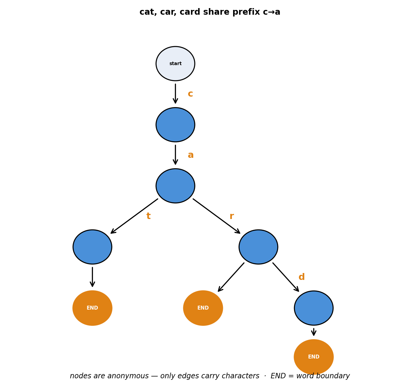
Nodes are anonymous — only the edges carry characters. Orange nodes mark word boundaries (END). The prefix c→a is stored once and shared by all three words. Lookup costs O(L) in the key length.
Mechanism trace — trie_insert("car") after "cat" already exists:
Before: trie = {'c': {'a': {'t': {'END': True}}}}
-
'c'intrie→ descend. Current node =trie['c']={'a': {'t': {'END': True}}}. -
'a'in node → descend. Current node ={'t': {'END': True}}. -
'r'not in node → create it. Node becomes{'t': {'END': True}, 'r': {}}. - Mark end. Node
'r'becomes{'END': True}.
After: trie = {'c': {'a': {'t': {'END': True}, 'r': {'END': True}}}}
Only 1 new node created. The shared prefix c→a cost nothing extra.
Costs: search/insert \(O(L)\) (\(L\) = key length, one \(O(1)\) dict lookup per character) · space \(O(\Sigma \cdot L_{\max} \cdot n)\) worst case (\(\Sigma\) = alphabet size, e.g. 26 for lowercase letters) but shared prefixes reduce this significantly.
D. Union-Find — group membership via parent pointers
Why · near-
O(1)per operation to track which group an element belongs to, across many merges. Where · merging duplicate records (entity resolution), clustering, Kruskal’s Minimum Spanning Tree algorithm (Graphs), connected components.
Union-Find is pointer-chained like a linked list, but every pointer points upward toward a
representative called the root. Instead of a next field in each node, there is one flat parent
array: parent[i] is the parent of element i. A root has parent[root] == root (it points to
itself).
Invariant: following any element’s parent pointers reaches a root. Two elements are in the same group if and only if they reach the same root.
Figure 5 · Union-Find: initial state, after two merges, after path compression.
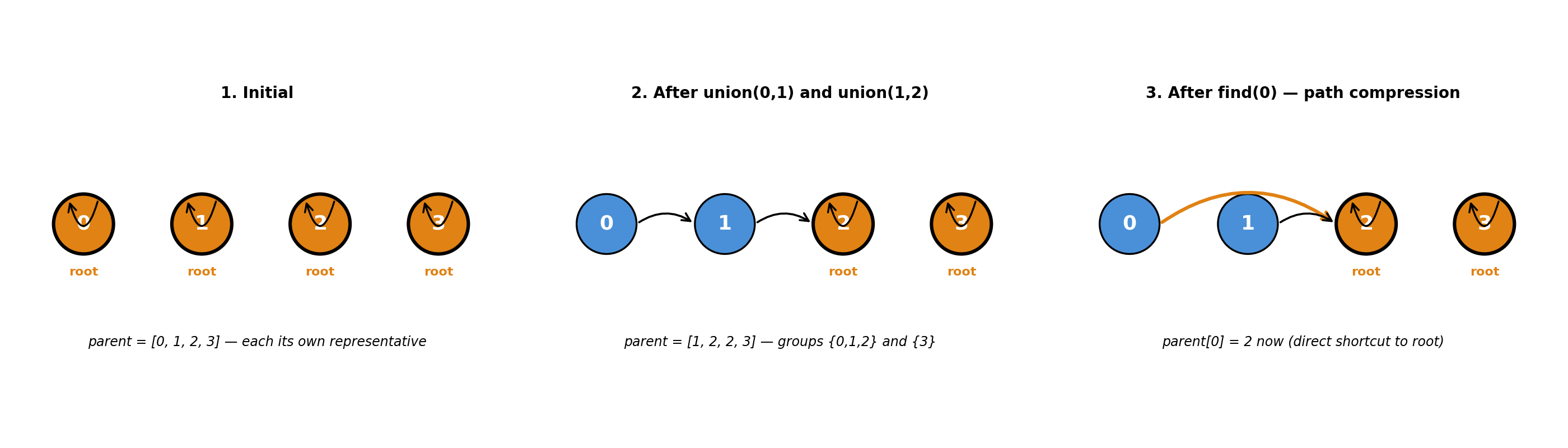
Panel 1: each element is its own root (all self-loops). Panel 2: after union(0,1) and union(1,2), the chain 0→1→2 forms one group; node 3 is alone. Panel 3: find(0) shortcuts 0 directly to root 2 (orange, path compression). The next find(0) costs one hop.
Example problem: given “connect A to B” operations, answer “are A and B in the same group?”
Algorithm:
parent = [0, 1, 2, 3]   # each element its own representative

def find(x):
    if parent[x] != x:
        parent[x] = find(parent[x])   # path compression
    return parent[x]

def union(x, y):
    root_x, root_y = find(x), find(y)
    if root_x != root_y:
        parent[root_x] = root_y

union(0, 1)
union(1, 2)
# parent = [1, 2, 2, 3]  — groups: {0,1,2} and {3}

find(0) == find(2)   # True
find(0) == find(3)   # False
Mechanism trace — same 4 elements as the figure:
-
union(0,1): root of 0 is 0, root of 1 is 1; setparent[0] = 1. (Figure panel 2, step 1.) -
union(1,2): root of 1 is 1, root of 2 is 2; setparent[1] = 2. Chain: 0→1→2. (Panel 2.) -
find(0): follow 0→1→2.parent[2]==2, stop. Path compression setsparent[0] = 2. (Panel 3.) - Next
find(0): one hop to root 2. O(1).
Costs: find/union \(O(\alpha(n))\) amortized · space \(O(n)\).
\(\alpha\) is the inverse Ackermann function. The Ackermann function grows absurdly fast, faster than any practical formula, so its inverse barely budges. \(\alpha(n) \leq 4\) for any \(n\) below \(A(4,4)\), a number with more digits than atoms in the observable universe. Mathematically it is not \(O(1)\), but you will never see it exceed 4.
Why nearly \(O(1)\): each node moves closer to the root at most once per level it traverses; after compression it points directly to the root and never contributes to a long path again. The total traversal work across all operations is bounded, giving \(O(\alpha(n))\) amortized rather than \(O(\log n)\).
🔗 Connections
- Linear structures (the two memory primitives these build on): Linear Structures.
- Master map and cost table: Overview.
- Heap used in Dijkstra and graph MST algorithms: Graphs.
- Heap used in heapsort: Sorting & Searching.
- Trie and Union-Find as recognition triggers: the upcoming pattern-triggers post.