2. Foundations

📐 How to reason about cost: Big-O, the master theorem, and loop invariants.

2026 · dsa-fundamentals big-o recursion master-theorem invariants complexity

A. Asymptotic notation: ignore constants, keep the shape

Why · compare algorithms without drowning in constants. Where · every cost cell in the atlas is written this way.

Compare by how fast cost grows as \(n\) gets large, ignoring constants and smaller terms. So \(10n\) and \(100n\) are both \(O(n)\): same shape, and the constant only changes the slope.

Notation	Bound	Read as
\(O(f)\)	upper	“grows no faster than \(f\)”
\(\Omega(f)\)	lower	“grows at least as fast as \(f\)”
\(\Theta(f)\)	tight	“grows exactly like \(f\)” (both \(O\) and \(\Omega\))

What is \(n\)? Input size, not value. An \(n\times n\) matrix has input size \(\Theta(n^2)\): every cell counts. (Graphs measure size as \(|V|+|E|\); see Graphs.)

Reading a cost cell: amortized ≠ worst. An amortized cost is the average over a run, not the worst single call. list.append is usually free, but when the list fills up it copies into a bigger block: one \(O(n)\) call. Since each resize doubles the capacity, those copies get rare enough that \(n\) appends total \(O(n)\), i.e. \(O(1)\) per append on average. That’s why the tables list it as amortized \(O(1)\).

B. The growth ladder: why the exponent matters

Why · turn a Big-O into a gut feel for “will this run in time?”. Where · deciding if code survives 100× data; the hidden-\(O(n^2)\) audit on the upcoming DSA-at-work post.

Fastest to slowest. At \(n=1000\) the gap runs from instant to impossible, so check the exponent first.

Class	Name	Ops at \(n=1000\)	Typical source
\(O(1)\)	constant	1	hash lookup, array index
\(O(\log n)\)	logarithmic	~10	binary search, balanced-tree op
\(O(n)\)	linear	1 000	one pass over input
\(O(n \log n)\)	linearithmic	~10 000	a good sort (merge / heap)
\(O(n^2)\)	quadratic	1 000 000	nested loop / missing hash set
\(O(2^n)\)	exponential	~\(10^{300}\)	all subsets (only \(\sim 10^{80}\) atoms exist)

Figure 1 · Growth curves with a time-budget ceiling (linear y-axis).

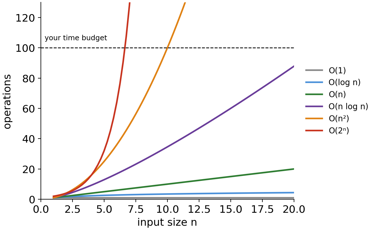
\(O(2^n)\) and \(O(n^2)\) punch through the budget line at \(n \approx 7\) and \(n \approx 10\), while the cheap classes barely lift off the floor. That gap is the whole subject.

Figure 2 · Largest \(n\) you can finish in time.

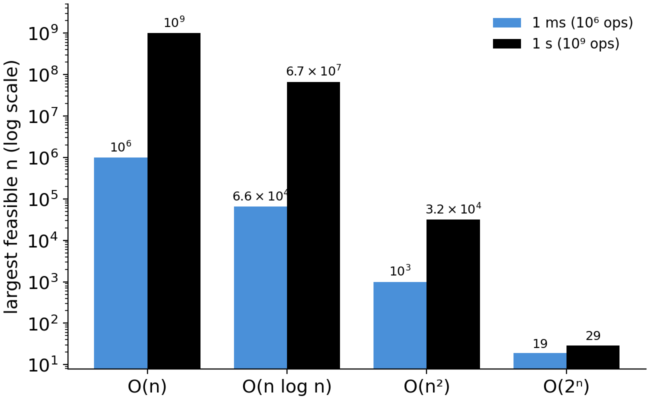
At ~1 ns/op, each class gets two bars: 1 ms (\(10^6\) ops) and 1 s (\(10^9\) ops). Even with a full second, quadratic stalls at \(n \approx 31{,}000\) and exponential dies before \(n=30\).

Gut check (the everyday transfer):

On a request path or a pipeline over millions of rows, \(O(n^2)\) is 🔴 dangerous, and usually a missing set/dict.
At \(n<100\) it doesn’t matter, so don’t optimize a once-a-week script. (See the upcoming pattern-triggers post / the upcoming DSA-at-work post.)

C. Recursion → cost: the master theorem as a lookup

Why · read a recursive algorithm’s cost without solving the recurrence by hand. Where · any divide-and-conquer: merge sort, binary search, the recursion on Sorting & Searching / Recursion & Backtracking.

A recursive algorithm’s cost is a recurrence: \(T(n) = a\,T(n/b) + f(n)\), i.e. a subproblems of size n/b, plus f(n) to split and recombine. Don’t solve it. Match the shape and read the answer off:

Compute \(n^{\log_b a}\) (the cost if all the work were at the leaves).
Compare \(f(n)\) to it:

Case	Condition	Result
1 · leaf-heavy	\(f(n)\) grows slower than \(n^{\log_b a}\)	\(T = \Theta(n^{\log_b a})\)
2 · balanced	\(f(n) = \Theta(n^{\log_b a}\log^k n)\)	\(T = \Theta(n^{\log_b a}\log^{k+1} n)\)
3 · root-heavy	\(f(n)\) grows faster	\(T = \Theta(f(n))\)

Strictly: “slower/faster” means polynomially so (by a factor \(n^\varepsilon\)), and Case 3 needs a regularity condition. Rare gap cases fall outside all three, but every case you’ll meet in practice fits.

Merge sort (split in two, recurse on each half, then an \(O(n)\) merge)

\[T(n) = 2\,T(n/2) + n\]

\(a=2\) (two subproblems), \(b=2\) (each half the size), \(f(n)=n\) (merge cost).
Leaf cost: \(n^{\log_b a} = n^{\log_2 2} = n^1 = n\).
Compare: \(f(n) = n = \Theta(n^1)\), which matches the leaf cost exactly → Case 2 (balanced).
Result: \(T(n) = \Theta(n \log n)\).

The full merge-sort algorithm lives on Sorting & Searching; here it’s only an example input to the theorem.

Figure 3 · Recursion tree for merge sort + the three master-theorem cases.

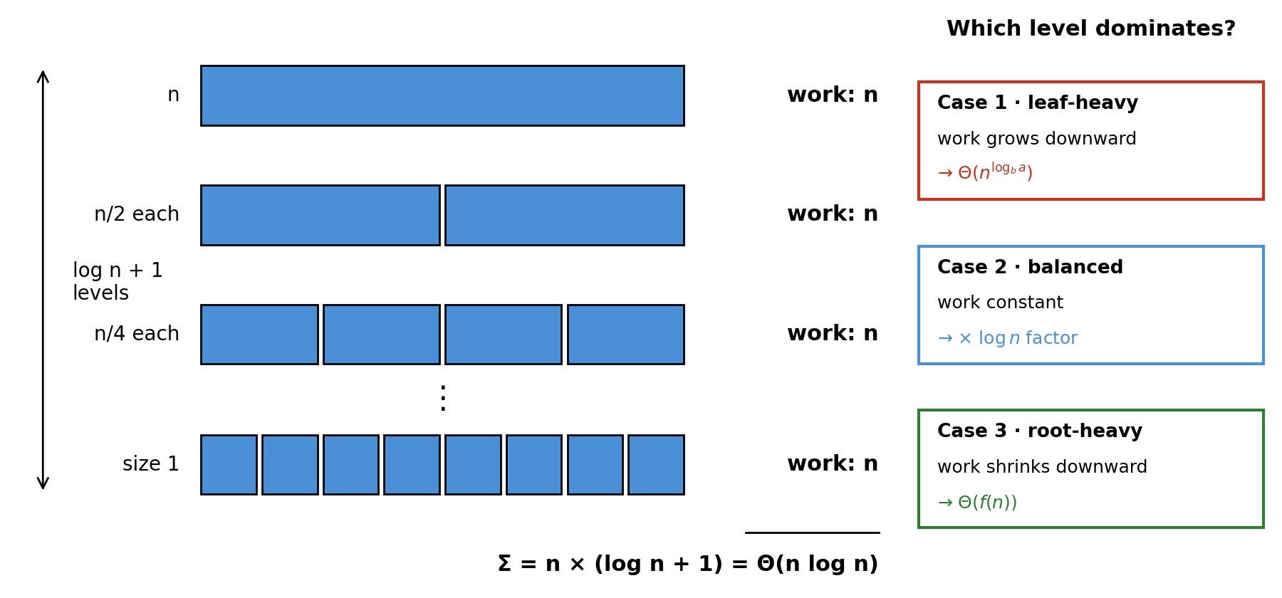
Left: each level costs \(n\); there are \(\log n + 1\) levels, so the total is \(\Theta(n \log n)\). Right: the three cases depend on whether per-level work grows, holds, or shrinks.

D. Invariants: the loop-correctness tool

Why · know a loop is right without tracing it. Where · binary search & sliding window, where off-by-ones live (full treatment there).

An invariant is a claim about your variables that stays true on every lap. Keep it true each lap and, at exit, the claim plus the stop condition hands you the answer, no tracing required. Three checks:

Start: it holds before the first lap.
Each lap: the body preserves it.
End: at termination it gives the result.

The whole skill is naming the right claim. Take binary search for 9 in [1, 4, 7, 9, 15], invariant: “if 9 is here, it’s in [lo, hi].”

Start: lo, hi = 0, 4 (the whole array). True by definition.
Lap 1: mid value is 7 < 9, so 7 and everything left of it can’t be the answer → lo = 3. Window is now [9, 15], and the claim still holds.
Lap 2: mid value is 9. Found it.
Why it’s safe: each lap drops only the half that can’t hold the target, so the claim never breaks, and the window shrinks to the answer (or lo > hi, meaning it was never there).

Full treatment on Sorting & Searching; the invariant idea is applied again on Array & String Techniques.

🔗 Connections

Master map: Overview.
Growth ladder → ranks every cost cell across the atlas.
Recurrences → explain the costs on Sorting & Searching (merge sort) and Recursion & Backtracking.
Invariants → justify the loops on Array & String Techniques and Sorting & Searching.

⏮ 1. Overview 3. Linear Structures ⏭