8. Graphs
🕸️ The capstone: representation, BFS/DFS, topological sort, shortest paths, and MST.
The unifying idea. A graph is a set of nodes connected by edges. Almost every “model relationships” problem reduces to one of five operations: represent the graph, traverse it (BFS/DFS), order it (topo sort), find cheapest paths (shortest paths), or find the cheapest spanning structure (MST). This sheet covers all five.
| Problem shape | Operation | Section |
|---|---|---|
| Model relationships between entities; choose how to store them | Representation | A |
| Visit all reachable nodes; find shortest path in unweighted graph; detect cycles | BFS / DFS | B |
| Schedule tasks with prerequisites; process in dependency order | Topological sort | C |
| Find minimum-cost path from one source to all other nodes | Shortest paths | D |
| Connect all nodes with minimum total edge weight, no cycles | MST | E |
A. Graph representations
Why · the right representation determines whether every operation is fast or slow. Where · any graph problem; choose before coding.
A graph \(G = (V, E)\) has vertices \(V\) and edges \(E\). Two standard representations:
Adjacency list — a dict mapping each node to its neighbors. Standard for sparse graphs.
# unweighted directed graph: 0→1, 0→2, 1→3, 2→3, 3→4
graph = {
    0: [1, 2],
    1: [3],
    2: [3],
    3: [4],
    4: [],
}

# weighted: each neighbor is a (node, weight) pair
weighted = {
    0: [(1, 2), (2, 6)],
    1: [(3, 8)],
    2: [(3, 3)],
}
Adjacency matrix — a 2D array where matrix[u][v] holds the edge weight (0 if no edge).
Standard for dense graphs or when \(O(1)\) edge lookup is required.
# same graph as a matrix (5 nodes)
matrix = [
    [0, 1, 1, 0, 0],   # node 0
    [0, 0, 0, 1, 0],   # node 1
    [0, 0, 0, 1, 0],   # node 2
    [0, 0, 0, 0, 1],   # node 3
    [0, 0, 0, 0, 0],   # node 4
]
Figure 1 · The same graph as an adjacency list and adjacency matrix.
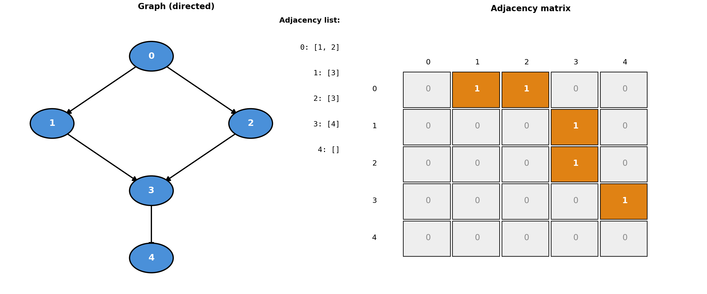
Orange cells in the matrix mark edges. The list only stores existing edges; the matrix stores all possible pairs — that difference drives the space and lookup costs.
Cost comparison:
| Adjacency list | Adjacency matrix | |
|---|---|---|
| Space | \(O(V + E)\) | \(O(V^2)\) |
Edge lookup (u,v)
|
\(O(\deg(u))\) — scan neighbors | \(O(1)\) — direct index |
| Iterate all edges | \(O(V + E)\) | \(O(V^2)\) |
Use list when the graph is sparse (\(E \ll V^2\)) — most real graphs. Use matrix when \(V\) is small and you need fast edge queries, or when the graph is dense.
B. BFS and DFS
Why · reach all nodes reachable from a source; differ in what order they visit nodes, which determines what each algorithm can guarantee. Where · BFS for shortest paths in unweighted graphs and level-order traversal; DFS for topo sort, cycle detection, and connected components.
Both algorithms visit every reachable node exactly once: \(O(V + E)\) — one pass over each vertex and each edge. The difference is the data structure that controls visit order.
Figure 2 · BFS wavefront vs DFS corridor on the same graph.
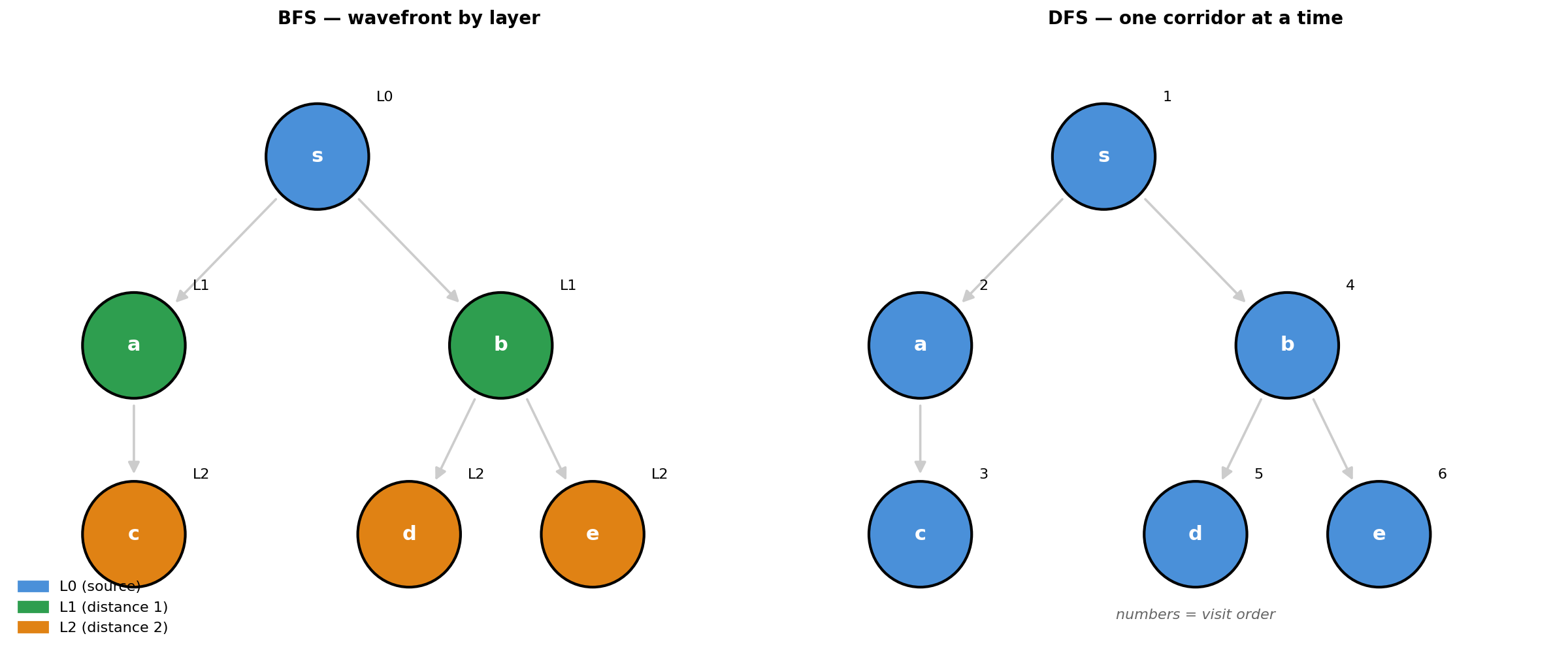
BFS (left): expands level by level — all nodes at distance \(k\) before any at \(k+1\). DFS (right): plunges down one path until stuck, then backtracks. Numbers show DFS visit order.
BFS — uses a queue; guarantees shortest path in unweighted graphs.
The queue is FIFO, so all nodes discovered at distance 1 are processed before any at distance 2,
and so on. A node is never revisited (if neighbor not in dist prevents it), so its distance is
fixed at the first — and therefore minimum — number of hops it took to reach it.
Invariant: all nodes at distance \(k\) from the source are fully processed before any node at distance \(k+1\) is visited.
from collections import deque

def bfs(graph, source):
    dist = {source: 0}
    queue = deque([source])
    while queue:
        node = queue.popleft()
        for neighbor in graph[node]:
            if neighbor not in dist:
                dist[neighbor] = dist[node] + 1
                queue.append(neighbor)
    return dist
Mechanism trace on the graph from Figure 2, source = s:
- Queue:. Visit s (dist=0). Enqueue a, b.
- Queue:
[a, b]. Visit a (dist=1). Enqueue c. - Queue:
[b, c]. Visit b (dist=1). Enqueue d, e. - Queue:
[c, d, e]. Visit c, d, e (dist=2). Queue empty → done.
Cost: \(O(V + E)\) — each node enqueued once, each edge examined once.
DFS — uses recursion (implicit stack); produces finish order used for topo sort.
The call stack naturally goes as deep as possible before backtracking. A node finishes (returns) only after all nodes reachable from it have been fully explored — deeper nodes finish first, shallower nodes last. Section C uses this finish order for topological sort.
Invariant: a node is marked finished only after all nodes reachable from it are finished.
def dfs(graph, source, visited=None):
    if visited is None:
        visited = set()
    visited.add(source)
    for neighbor in graph[source]:
        if neighbor not in visited:
            dfs(graph, neighbor, visited)
    return visited   # reachability only; Section C extends this to record finish order
Mechanism trace on Figure 2, source = s:
- Visit s → recurse into a.
- Visit a → recurse into c.
- Visit c → no unvisited neighbors → c finished.
- Back at a → no more neighbors → a finished.
- Back at s → recurse into b → visit b, d, e in order → b finished → s finished.
Cost: \(O(V + E)\) — each node visited once, each edge examined once.
| BFS | DFS | |
|---|---|---|
| Data structure | Queue | Recursion / stack |
| Order | Level by level (wavefront) | Deep first (corridor) |
| Shortest path (unweighted) | ✓ | ✗ |
| Topo sort / cycle detection | ✗ | ✓ |
| Connected components | ✓ | ✓ |
Note: Floyd’s cycle detection (fast/slow pointer) is a related technique for detecting cycles in linked structures (not a graph traversal algorithm) — see Array & String Techniques.
C. Topological sort
Why · produce a linear ordering of nodes such that for every edge A → B, A appears before B — so no dependency is ever processed before the thing it depends on. Where · task scheduling, dependency resolution, build systems, DAG DP.
A topological order of a directed acyclic graph (DAG) is a sequence of nodes where every directed edge \(u \to v\) has \(u\) before \(v\). It exists if and only if the graph is a DAG (no cycles).
Intuition — built up step by step:
- Finish time encodes dependency depth: DFS fully explores a node’s dependencies before marking it finished. Leaf nodes (no outgoing edges) finish first; a source node with many downstream dependencies finishes last, because its entire subtree must complete first.
- Reverse finish order = topo order: if there is an edge \(u \to v\), DFS finishes \(v\) before \(u\) (it recurses into \(v\) first). Reversing puts \(u\) before \(v\) — exactly the topological requirement.
Invariant: a node appears in the output only after all nodes it depends on have been output.
Figure 3 · Course prerequisite DAG: DFS finish times and one valid topo order.
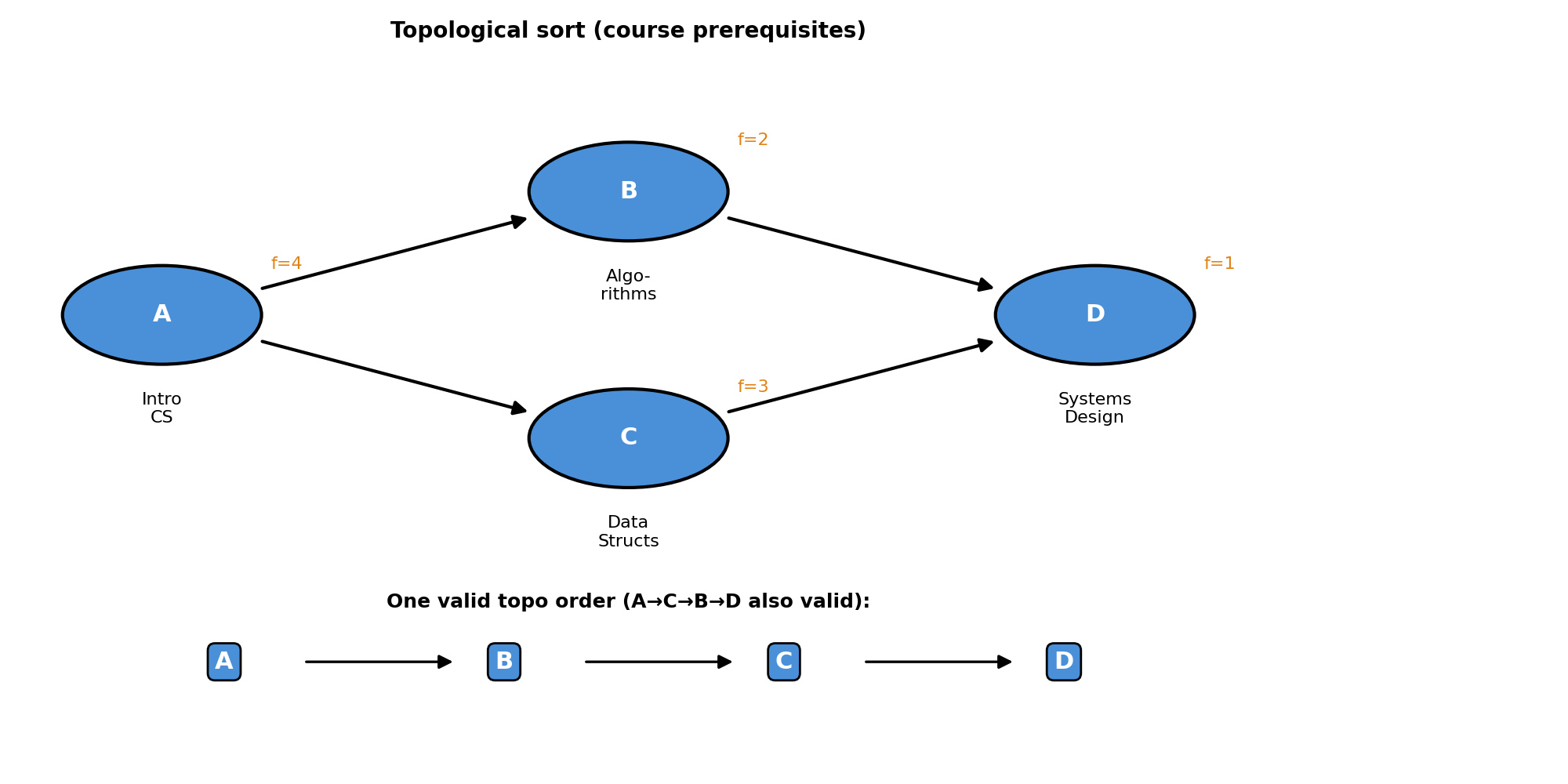
Diamond shape: A must precede B and C; both B and C must precede D. Two valid orders exist (A→B→C→D or A→C→B→D) — topo sort finds one. Finish times (\(f=\)) annotate each node; reversing them gives the order.
Algorithm:
def topo_sort(graph):
    visited = set()
    result = []

    def dfs(node):
        visited.add(node)
        for neighbor in graph[node]:
            if neighbor not in visited:
                dfs(neighbor)
        result.append(node)          # finish: all dependencies done

    for node in graph:
        if node not in visited:
            dfs(node)
    return result[::-1]             # reverse = topo order
Mechanism trace on Figure 3 (A=Intro CS, B=Algorithms, C=Data Structs, D=Systems Design):
- DFS from A → recurse into B → recurse into D.
- D has no neighbors → D finishes (f=1). Append D.
- Back at B → no more neighbors → B finishes (f=2). Append B.
- Back at A → recurse into C → D already visited → C finishes (f=3). Append C.
- Back at A → no more neighbors → A finishes (f=4). Append A.
- Reverse:
[A, B, C, D]— A before B and C, both before D. ✓
B finishes before C only because B appears first in A’s adjacency list — there is no dependency between B and C, so both orderings are equally valid. The algorithm picks one arbitrarily based on iteration order.
Cost: \(O(V + E)\) — one full DFS pass.
[DP expansion — ~2 lines] Topological order enables DAG DP: process nodes in topo order so each node’s subproblem is solved after all its dependencies. Shortest/longest paths in a DAG, counting paths, and many scheduling problems reduce to this. Add memoization here → that’s Dynamic Programming, deliberately deferred from this atlas.
D. Shortest paths
Why · find the minimum-cost path from a source to all other nodes. Where · routing, navigation, network cost optimization, any “minimum cost to reach” problem.
Problem: given a weighted graph \(G = (V, E, w)\) and source node \(s\), find the shortest-path distance \(\delta(s, v)\) from \(s\) to every node \(v \in V\), where \(\delta(s, v)\) is the minimum total weight over all paths from \(s\) to \(v\) (\(\infty\) if \(v\) is unreachable).
Relaxation is the shared core operation across all SSSP algorithms. Every node starts with distance estimate \(d[v] = \infty\) — “I don’t know how to reach you yet” — except the source \(d[s] = 0\). Relaxing edge \((u, v, w)\) asks: “is the path through \(u\) — costing \(d[u] + w\) — cheaper than my current best \(d[v]\)?” If yes, update. Estimates only ever decrease, never overshoot. Repeat until no more updates are possible and every \(d[v]\) converges to \(\delta(s, v)\). The algorithms below differ only in the order they choose to relax edges, which determines their cost and which graphs they handle correctly.
def relax(u, v, w, dist):
    if dist[u] + w < dist[v]:   # cheaper path to v found via u?
        dist[v] = dist[u] + w   # tighten the estimate
Figure 4 · Relaxation on a 3-node graph: the cheaper path via u beats the direct s→v edge.
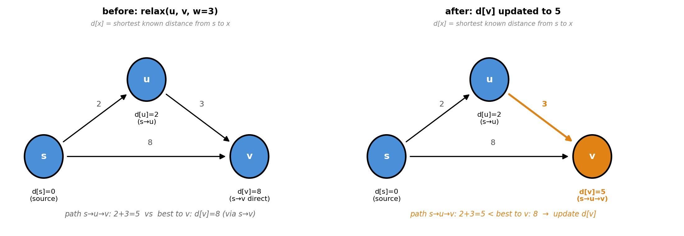
d[u]=2 was already set via s→u. Relaxing u→v asks: is 2+3=5 cheaper than the current d[v]=8 (set via s→v direct)? Yes → d[v] updates to 5 (orange). The condition and update are identical in every SSSP algorithm — only the order of relaxations differs.
Which algorithm? — depends on the graph type:
| Graph type | Edge weights | Algorithm | Cost |
|---|---|---|---|
| Unweighted | all = 1 | BFS (Section B) | \(O(V + E)\) |
| DAG | any | DAG relaxation | \(O(V + E)\) |
| General | non-negative | Dijkstra | \(O((V + E) \log V)\) |
| General | any (negative ok) | Bellman-Ford | \(O(V \cdot E)\) |
Dijkstra’s algorithm — general graphs with non-negative weights.
Intuition — built up step by step:
-
The heap is a min-heap of
(distance, node)pairs. It starts with just the source at distance 0. The minimum is always at the root, so the next candidate costs \(O(1)\) to read and \(O(\log V)\) to remove (one swap per level as the heap sifts down to restore order). - Settling a node means: pop it from the heap, declare its distance final, then relax all its outgoing edges — for each neighbor, check if going through this node beats the current best known distance, and if so push the improved estimate onto the heap.
- Why the distance is final when settled: the heap always gives the smallest current estimate next. Any future path to this node would go through an unsettled node, which has distance at least as large — so it can only be equal or worse. Negative weights break this: a negative edge discovered later could shorten a distance already declared final.
- The sphere: settling always expands to the nearest unsettled node, so the settled set grows outward by distance — like a wavefront.
Invariant: once a node is settled, its distance is the true shortest-path distance.
Figure 5 · Dijkstra sphere growing: settled nodes (green), frontier (blue), unseen (grey).
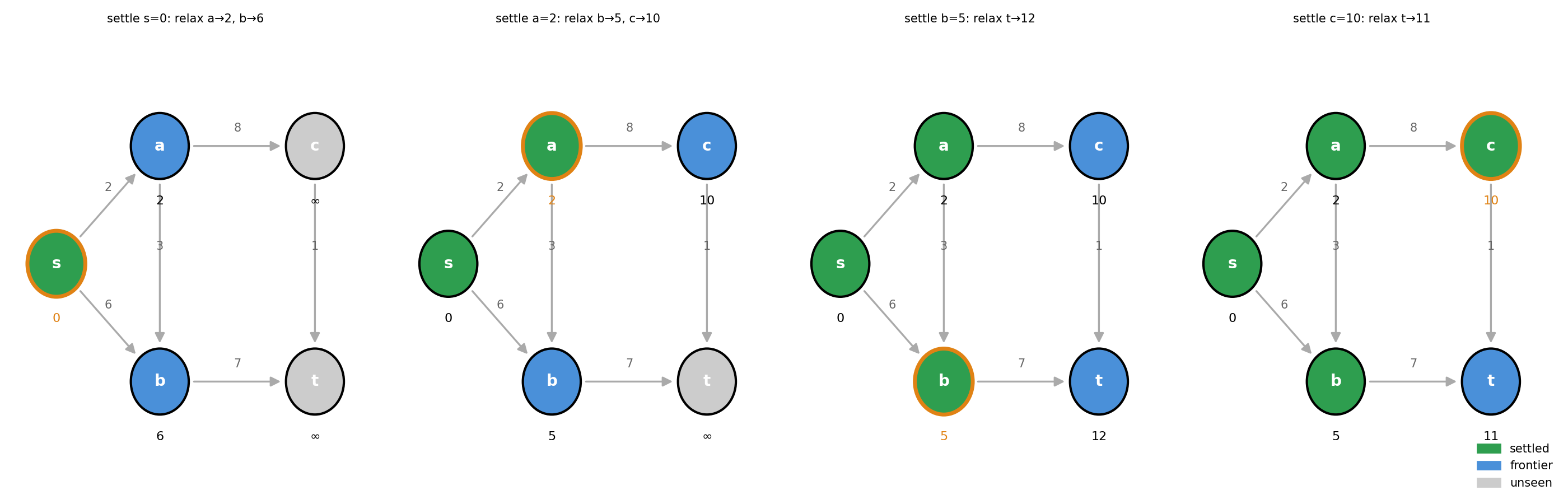
Each panel settles one node (orange border). Distances below each node update as relaxations tighten estimates. The sphere grows outward from s.
Algorithm:
import heapq

def dijkstra(graph, source):
    dist = {node: float("inf") for node in graph}
    dist[source] = 0
    heap = [(0, source)]               # (distance, node)

    while heap:
        d, node = heapq.heappop(heap)
        if d > dist[node]:
            continue                   # stale entry — already settled
        for neighbor, weight in graph[node]:
            new_dist = dist[node] + weight
            if new_dist < dist[neighbor]:
                dist[neighbor] = new_dist
                heapq.heappush(heap, (new_dist, neighbor))
    return dist
Mechanism trace on Figure 5, edges as shown:
- Pop (0,s) → settle s (dist=0): relax a→2, b→6. Heap:
[(2,a),(6,b)]. - Pop (2,a) → settle a (dist=2): relax b→5 (improves 6→5), c→10. Heap:
[(5,b),(6,b),(10,c)]. - Pop (5,b) → settle b (dist=5): relax t→12. Heap:
[(6,b),(10,c),(12,t)]. - Pop (10,c) → settle c (dist=10): relax t→11 (improves 12→11). Heap:
[(11,t),(12,t)]. - Pop (11,t) → settle t (dist=11). Done. Result:
{s:0, a:2, b:5, c:10, t:11}.
(Steps 4–5 skip stale entries (6,b) and (12,t) along the way — nodes already settled get
popped and discarded by the if d > dist[node]: continue guard.)
Cost: \(O((V + E) \log V)\) — each node popped once (\(V\) pops), each edge relaxed once (\(E\) pushes), each heap operation costs \(O(\log V)\).
Bellman-Ford — handles negative edge weights; detects negative cycles.
Intuition — built up step by step:
- No ordering assumption: unlike Dijkstra, Bellman-Ford does not pick the closest node next. It relaxes every edge in the graph, in any order, once per round.
- Why \(V - 1\) rounds: after round \(k\), every node whose shortest path uses at most \(k\) edges has the correct distance. A simple path (no repeated nodes) uses at most \(V - 1\) edges, so \(V - 1\) rounds guarantee all estimates have converged.
- Negative cycles: if a \(V\)-th round still relaxes some edge, then there exists a path that keeps getting cheaper by going around a cycle with negative total weight. No finite shortest distance exists in that case.
Invariant: after round \(k\), \(d[v]\) holds the true shortest distance from \(s\) to \(v\) using at most \(k\) edges.
Figure 6 · Bellman-Ford: distance estimates converging over three rounds.
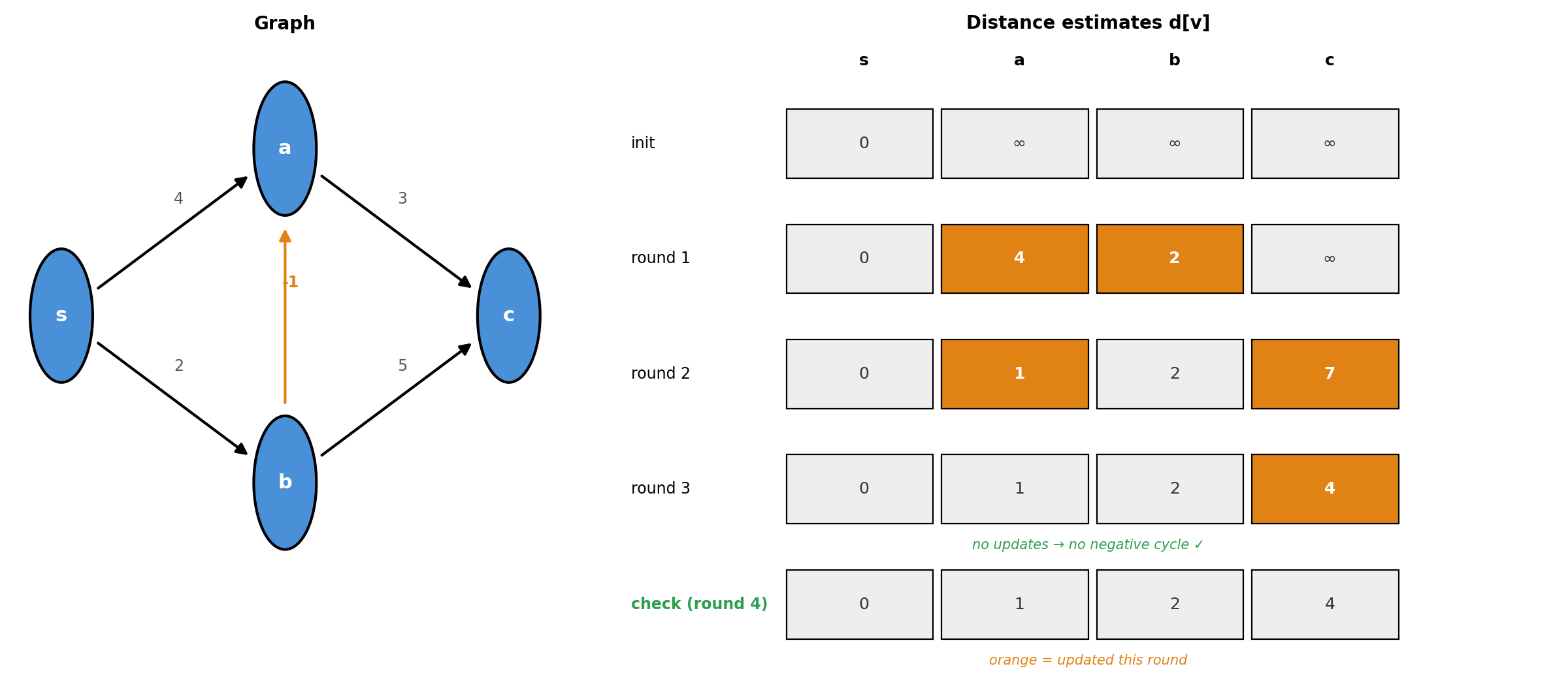
Left: the graph (orange = negative edge). Right: each row is one round; orange cells show updated values. After V−1 rounds all estimates have converged. A further round that still updates signals a negative cycle.
def bellman_ford(nodes, edges, source):
    dist = {node: float("inf") for node in nodes}
    dist[source] = 0

    for _ in range(len(nodes) - 1):    # V-1 rounds
        for u, v, w in edges:          # relax every edge
            if dist[u] + w < dist[v]:
                dist[v] = dist[u] + w

    for u, v, w in edges:              # check for negative cycle
        if dist[u] + w < dist[v]:
            raise ValueError("negative cycle detected")
    return dist
Mechanism trace: see Figure 6 — the table shows each round’s updates more clearly than prose steps.
Cost: \(O(V \cdot E)\) — \(V - 1\) rounds each examining all \(E\) edges.
Johnson’s algorithm — all-pairs shortest paths (pointer, not covered in full).
Problem: find \(\delta(u, v)\) for every pair \((u, v) \in V \times V\) — not just from one source.
Why not just run Dijkstra from every node? Dijkstra requires non-negative weights. On graphs with negative edges, running it from every node is incorrect.
Why not run Bellman-Ford from every node? That works but costs \(O(V^2 \cdot E)\) — too slow.
Johnson’s trick — built up step by step:
- Add a dummy source \(q\) with zero-weight edges to every node. Run Bellman-Ford once from \(q\) to get \(h(v) = \delta(q, v)\) for every node — the potential of \(v\), i.e. its shortest distance from the dummy source.
- Reweight every edge: \(\hat{w}(u,v) = w(u,v) + h(u) - h(v)\). This shifts the original weight by the difference in shortest-path distances from the dummy source to the two endpoints. The triangle inequality guarantees \(h(v) \leq h(u) + w(u,v)\), so \(\hat{w}(u,v) \geq 0\). Along any path, the \(h\) terms telescope — every intermediate node’s \(h\) cancels between consecutive edges — so all paths between the same pair \((s, t)\) shift by the same constant \(h(s) - h(t)\), preserving which path is shortest.
- Run Dijkstra from every node on the reweighted graph. Recover original distances: \(\delta(u,v) = \hat{\delta}(u,v) - h(u) + h(v)\).
Cost: \(O(VE)\) for Bellman-Ford + \(O(V \cdot (V+E) \log V)\) for \(V\) Dijkstra runs \(= O(V^2 \log V + VE)\). Running Bellman-Ford from every node would cost \(O(V^2 E)\), so Johnson’s is faster by a factor of \(E / (V \log V + E)\) — most significant on dense graphs where \(E \approx V^2\), giving a factor of \(\approx V\).
E. Minimum spanning tree
Why · connect all nodes with the minimum total edge weight and no cycles — the cheapest network that keeps everything reachable. Where · network design, clustering, Kruskal’s is also the canonical Union-Find application.
A spanning tree of a connected graph is a subset of edges that connects all nodes with no cycles — exactly \(V - 1\) edges for \(V\) nodes. Many spanning trees exist; the minimum one has the smallest total edge weight.
Problem: given a connected undirected weighted graph \(G = (V, E, w)\), find a spanning tree \(T \subseteq E\) that minimises \(\sum_{e \in T} w(e)\).
Figure 7 · A weighted graph (left) and its minimum spanning tree (right).
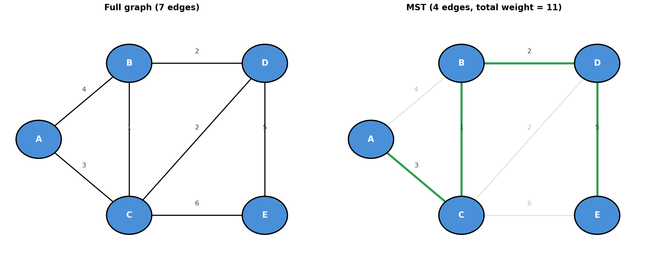
Left: all edges with weights. Right: the MST (green) connects all 5 nodes with 4 edges at minimum total weight. Dropped edges (grey) would create cycles or aren’t needed.
Two greedy algorithms solve this — each makes one irrevocable choice per step and never backtracks. Greedy works for MST because of the cut property: partition the nodes into any two groups; the cheapest edge crossing that partition must be in the MST. Why? If the MST used a more expensive crossing edge instead, you could swap it for the cheaper one, reduce total weight, and still have a spanning tree — contradicting minimality. This means any algorithm that repeatedly picks the cheapest “safe” edge (one that doesn’t form a cycle) is guaranteed to produce the MST.
Both algorithms below exploit the cut property with a different strategy and a different structure from Hierarchical Structures: Kruskal processes edges globally by weight (Union-Find detects cycles), Prim grows a frontier locally (min-heap picks the cheapest crossing edge).
Kruskal’s algorithm — sort all edges by weight; add each if it doesn’t create a cycle. Uses Union-Find (see Hierarchical Structures Section D) to detect cycles in near-\(O(1)\).
Intuition — built up step by step:
- Greedy by edge weight: the globally cheapest edge that doesn’t create a cycle is always safe to add to the MST. Processing all edges in sorted order applies this greedily.
- Cycle detection via Union-Find: two nodes are in the same connected component if they share a root in the Union-Find structure. Adding an edge between two nodes in the same component would close a cycle — skip it.
- Termination: stop when \(V - 1\) edges have been added. Exactly \(V - 1\) edges connect \(V\) nodes without cycles.
Invariant: the edges added so far form a spanning forest (multiple disconnected trees that haven’t merged yet) of minimum weight — no cheaper set of edges connects the same components. At termination the forest becomes a single spanning tree.
Figure 8 · Kruskal adding edges in sorted order; red = rejected (would create cycle).
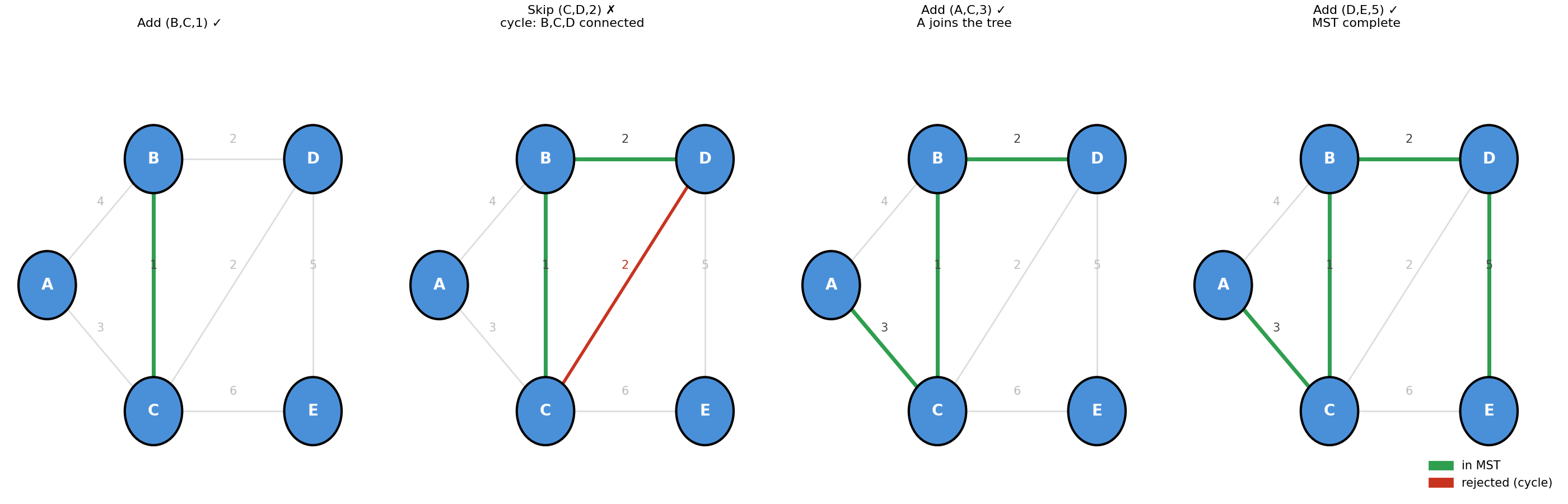
Panel 1: first add. Panel 2: (C,D,2) rejected — B, C, D already connected. Panel 3: (A,C,3) connects the isolated node A to the tree. Panel 4: (D,E,5) completes the MST.
def kruskal(nodes, edges):
    parent = {n: n for n in nodes}

    def find(x):
        if parent[x] != x:
            parent[x] = find(parent[x])   # path compression
        return parent[x]

    def union(x, y):
        parent[find(x)] = find(y)

    mst = []
    for u, v, w in sorted(edges, key=lambda e: e[2]):
        if find(u) != find(v):            # no cycle
            union(u, v)
            mst.append((u, v, w))
    return mst
Mechanism trace (nodes A–E, same graph as Figure 7):
- Sort edges: (B,C,1), (B,D,2), (C,D,2), (A,C,3), (D,E,5), (A,B,4), (C,E,6).
- Add (B,C,1) — no cycle. MST:
[(B,C,1)]. - Add (B,D,2) — no cycle. MST:
[(B,C,1),(B,D,2)]. - Add (C,D,2) — B,C,D already connected → skip cycle.
- Add (A,C,3) — no cycle. MST:
[..,(A,C,3)]. - Add (D,E,5) — no cycle. MST complete (4 edges for 5 nodes). ✓
Cost: \(O(E \log E)\) — sorting all \(E\) edges costs \(O(E \log E)\); each of the \(E\) Union-Find operations (find + union) costs near-\(O(1)\) amortized with path compression, so sorting dominates.
Prim’s algorithm — grow from one node; always add the cheapest edge crossing the frontier. Uses a min-heap (see Hierarchical Structures Section B).
Intuition — built up step by step:
- The frontier is the set of edges that cross from the already-settled MST nodes to unsettled nodes. At each step, the cheapest such edge is the safe greedy choice.
-
The heap stores
(weight, neighbor, parent)triples for all frontier edges. The root is always the cheapest crossing edge, giving \(O(1)\) access and \(O(\log V)\) removal. - Adding a node: pop the cheapest frontier edge, add its target to the MST, then push all edges leaving that newly added node onto the heap as new frontier candidates.
-
Stale entries: a node may appear in the heap multiple times with different weights as
better paths are discovered. The
if node in in_mst: continueguard skips the stale ones.
Invariant: the settled nodes and their connecting edges always form a minimum spanning tree of the subgraph induced by those nodes.
Figure 9 · Prim growing the MST step by step from node A.
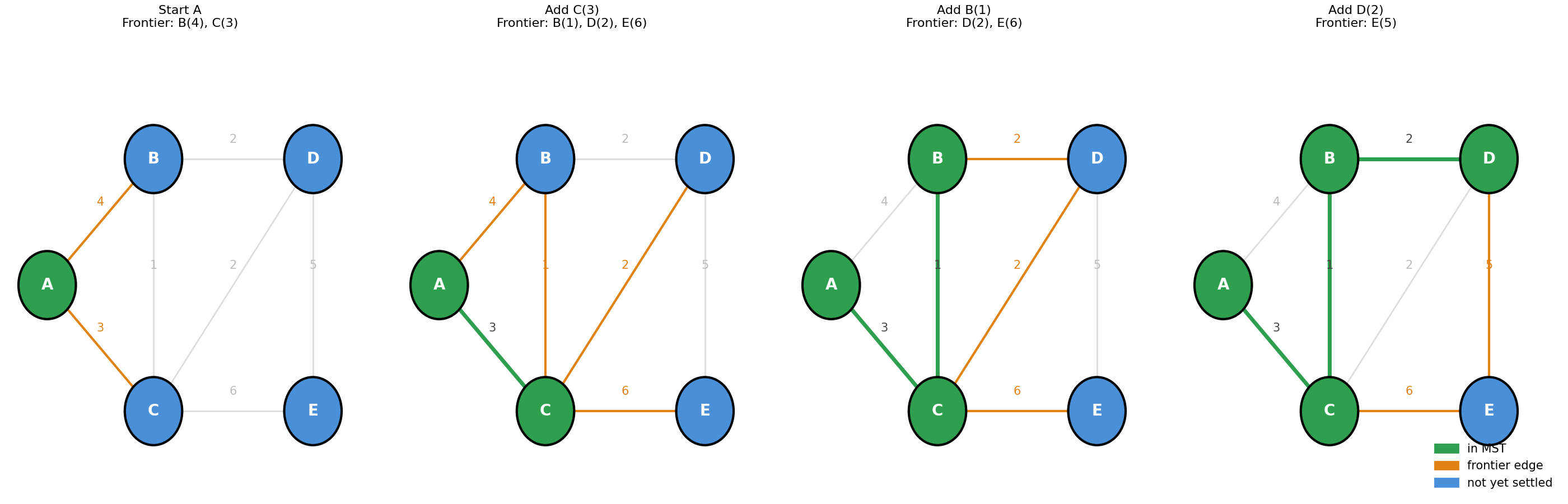
Green = in MST, orange = current frontier edges, blue = not yet reached. Each step the heap picks the cheapest frontier edge and the reached node joins the MST.
def prim(graph, start):
    in_mst = set()
    mst = []
    heap = [(0, start, start)]         # (weight, node, parent)

    while heap:
        w, node, parent = heapq.heappop(heap)
        if node in in_mst:
            continue
        in_mst.add(node)
        if node != start:
            mst.append((parent, node, w))
        for neighbor, weight in graph[node]:
            if neighbor not in in_mst:
                heapq.heappush(heap, (weight, neighbor, node))
    return mst
Mechanism trace on Figure 9, start = A:
- Settle A. Frontier: edges to B(4), C(3).
- Cheapest crossing edge: (A,C,3). Settle C. Frontier adds B(1 via C), D(2 via C), E(6).
- Cheapest: (C,B,1). Settle B. Frontier adds D(2 via B).
- Cheapest: (B,D,2) or (C,D,2) — tie, take (B,D,2). Settle D. Frontier adds E(5 via D).
- Cheapest: (D,E,5). Settle E. MST complete. ✓
Cost: \(O((V + E) \log V)\) — \(V\) nodes are popped from the heap (one settle per node), and up to \(E\) edges are pushed as frontier candidates. Each push and pop costs \(O(\log V)\), so total: \((V + E) \times O(\log V)\).
| Algorithm | Approach | Key structure | Cost |
|---|---|---|---|
| Kruskal | Sort edges, add if no cycle | Union-Find | \(O(E \log E)\) |
| Prim | Grow from one node via frontier | Min-heap | \(O((V+E) \log V)\) |
Use Kruskal when \(E\) is small (sparse graphs) — sorting is cheap and you can enumerate all edges. Use Prim when the graph is dense or already stored as an adjacency list — it settles one node at a time without needing all edges upfront.
🔗 Connections
- BFS uses deque from Linear Structures; DFS uses recursion stack from Recursion & Backtracking.
- Dijkstra and Prim use the min-heap from Hierarchical Structures.
- Kruskal uses Union-Find from Hierarchical Structures.
- Topo sort enables DAG DP — DP deliberately deferred from this atlas.
- Shortest-path decision table and graph recognition triggers: the upcoming pattern-triggers post.
- Floyd’s cycle detection (fast/slow pointer variant of traversal): Array & String Techniques.
- Kruskal used in MST; merge sort used in edge sorting: Sorting & Searching.