3. Linear Structures
🧱 The workhorse containers: dynamic array, hash map/set, linked list, stack, deque.
Two memory primitives. Every structure here is built on one of two layouts. Costs follow from the layout. Read the figure, read the cost:
| Primitive | Memory layout | Access | Insert/delete at known position |
|---|---|---|---|
| Contiguous | Elements packed at consecutive addresses: \(\text{addr}(i)=\text{base}+i\cdot s\) | \(O(1)\) | \(O(n)\), must shift neighbors |
| Pointer-chained | Elements anywhere; each node stores a next address |
\(O(n)\), follow \(i\) pointers | \(O(1)\), rewire two pointers |
The same two primitives power the hierarchical structures on Hierarchical Structures: BST, trie, and Union-Find are pointer-chained; the heap is contiguous.
A. Dynamic array: the contiguous primitive
Why · \(O(1)\) index and amortized \(O(1)\) append: the default container. Where · any time you need positional access or grow a sequence from the right end.
Figure 1 · Array memory layout: O(1) access and O(n) front insert.
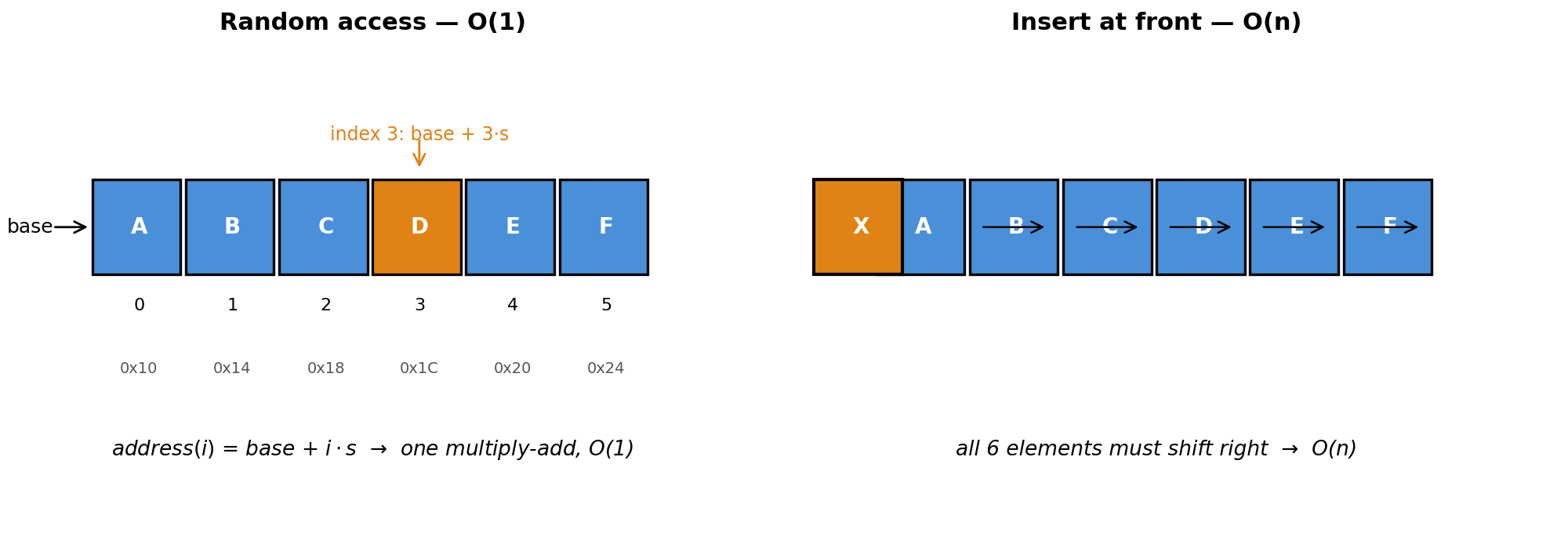
Left: \(\text{addr}(i) = \text{base} + i \cdot s\), one arithmetic op, no pointer chasing. Right: inserting at the front shifts every element right by one, unavoidable with contiguous memory.
Mechanism trace: a.append(x).
Fast path (size < capacity):
- Write
xat indexsize, incrementsize. Done: \(O(1)\).
Slow path (size == capacity, array is full):
- Allocate a new block of size \(2m\).
- Copy all \(m\) elements across. Costs \(O(m)\), once.
- Write
x, setcapacity = 2m, incrementsize.
Why the slow path doesn’t ruin the average:
Resizes happen at sizes \(1, 2, 4, \ldots, n\). Total copy work across all of them:
\[1 + 2 + 4 + \cdots + n \;=\; n\!\left(1 + \tfrac{1}{2} + \tfrac{1}{4} + \cdots\right) < 2n\](geometric series with ratio \(\frac{1}{2}\), sum converges to 2). Spread across \(n\) appends: \(\frac{2n}{n} = O(1)\) per append on average → amortized \(O(1)\).
Costs: access \(O(1)\) · search \(O(n)\) · append \(O(1)\)* · insert/delete at front \(O(n)\).
Use when: you index by position or append to the right end. Avoid for: repeated front insertions; use a deque (Section D).
B. Linked list: the pointer-chained primitive
Why · \(O(1)\) insert/delete at any known position, no shifting. Where · the mental model behind deque internals and pointer-manipulation problems.
Each element lives in a node: {item, next} where next is the memory address of the following
node. Nodes sit at arbitrary addresses; the chain is only in the pointers, not in memory layout.
Figure 3 · Linked-list memory layout: non-contiguous nodes, pointer chain.
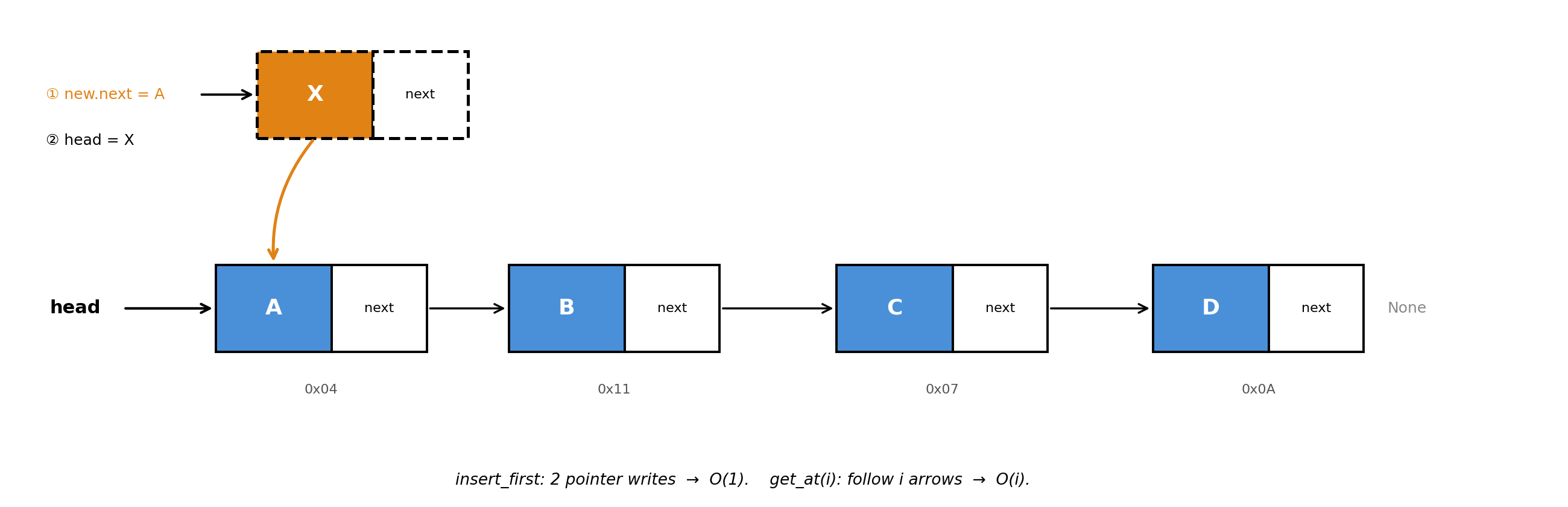
Addresses 0x04 → 0x11 → 0x07 → 0x0A: non-consecutive, only pointers connect them. New node X inserts with two pointer writes: ① new.next = head, ② head = new.
Mechanism trace: insert_first(x) (from the 6.006 notes).
- Allocate new node
NwithN.item = x. -
N.next = head: new node points to old first. -
head = N: list now starts at the new node. - Two pointer writes, regardless of list length → \(O(1)\).
Mechanism trace: get_at(i).
- Start at
head. - Follow
.nextpointers \(i\) times. - Return
node.item. \(O(i)\): must traverse, no shortcut.
Costs: insert/delete at known node \(O(1)\) · access by index \(O(n)\) · search \(O(n)\).
Python has no standalone linked list; collections.deque is backed by a linked structure and is what
you actually use. Reversal and Floyd’s cycle detection live on Array & String Techniques.
Use when: front insertions are the bottleneck. Not for indexing.
C. Stack: array, one end only
Why · \(O(1)\) push/pop; a dynamic array with one self-imposed constraint. Where · matching/nesting, DFS frontier (Graphs), undo.
A stack is a dynamic array (list) with one rule: only touch index \(n-1\) (the top). Last in, first
out. Since push is append and pop is list.pop(), both are amortized \(O(1)\) by the same doubling
argument as Section A.
Figure 4 · Stack layout: array with a top pointer.
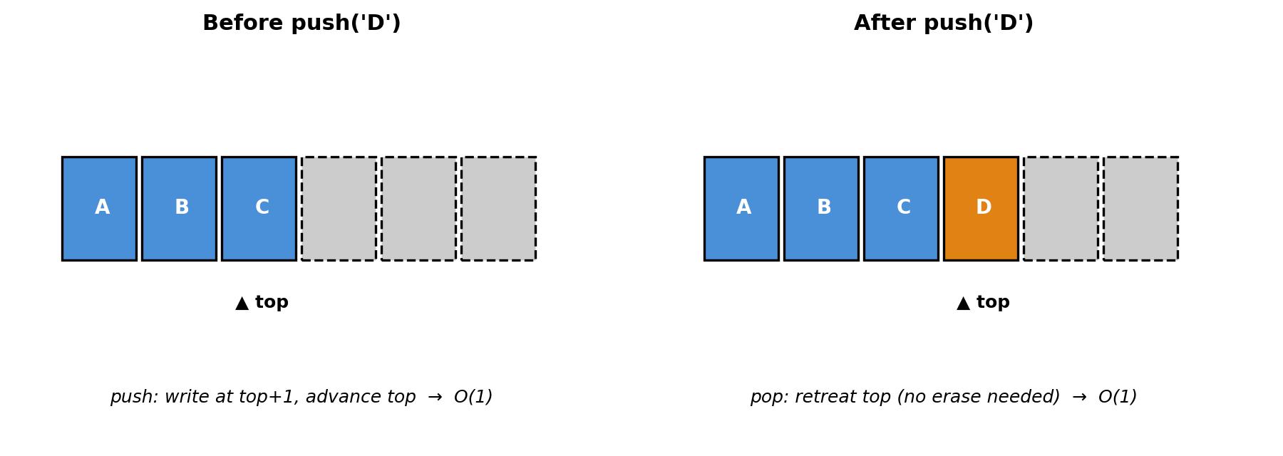
Before push: top sits at index 2, stack = [A, B, C]. After push(‘D’): top advances to index 3, one write. Pop simply retreats top, no memory erasure needed.
Mechanism trace: push and pop on [A, B, C].
-
push('D'): write'D'at index 3, top = 3. Stack =[A, B, C, D]. \(O(1)\). -
pop(): readstack[3]='D', decrement top to 2. Returns'D'. \(O(1)\). - Top always points to the last element: one read or write, no shifting.
Application: matching "(())" with a stack.
Rule: opening bracket → push it. Closing bracket → pop the top and check it matches. If the stack is empty when you need to pop, or non-empty at the end, the string is invalid.
| step | char | action | stack after | why |
|---|---|---|---|---|
| 1 | ( |
push | ['('] |
opening → remember it |
| 2 | ( |
push | ['(', '('] |
opening → remember it |
| 3 | ) |
pop → '('
|
['('] |
closing → the last-opened was (, matches ✓ |
| 4 | ) |
pop → '('
|
[] |
closing → the last-opened was (, matches ✓ |
| 5 | end | stack empty | n/a | all brackets paired → valid |
The stack naturally enforces the last opened must be the first closed, exactly the LIFO property.
Costs: push/pop \(O(1)\)* · peek stack[-1] \(O(1)\) · search \(O(n)\).
Use when: you need to process items in reverse-arrival order or track “what was the last open thing?”
D. Deque: linked blocks, both ends
Why · \(O(1)\) at both ends, which a plain list cannot match for front operations. Where · BFS queues (Graphs), sliding-window buffers (Array & String Techniques).
A deque (collections.deque) is a linked list of fixed-size blocks (like Section B, but each “node” is an array of ~8 elements). Two pointers, head (front block + offset) and tail (back block + offset), give \(O(1)\) access at either end.
Figure 5 · Deque layout: linked blocks with head/tail offsets.
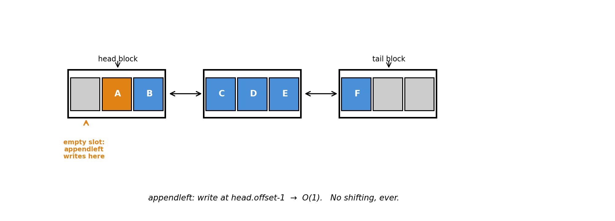
Three blocks linked like a linked list. The grey cell in the head block is reserved empty space: appendleft writes there and decrements the offset pointer. One write, no shifting, no allocation.
Mechanism trace: appendleft('X') on the deque from the figure (head block = [_, A, B], offset=1).
Slot available, \(O(1)\):
- Free slot exists at
head.offset - 1(the_position). - Write
'X'there, decrement offset to 0. Head block =[X, A, B]. One write, done.
Block full, still \(O(1)\):
- Allocate one new block, link it as the new head.
- Write
'X'into the new block. One allocation, one write.
Contrast, list.insert(0, 'X') on [A, B, C, D, E]:
- Every element shifts: \(a[i] \leftarrow a[i-1]\) for \(i = n-1, \ldots, 1\).
- Write
'X'at index 0. \(O(n)\), unavoidable with contiguous memory.
Figure 6 · Front insertion: list O(n) vs deque O(1).
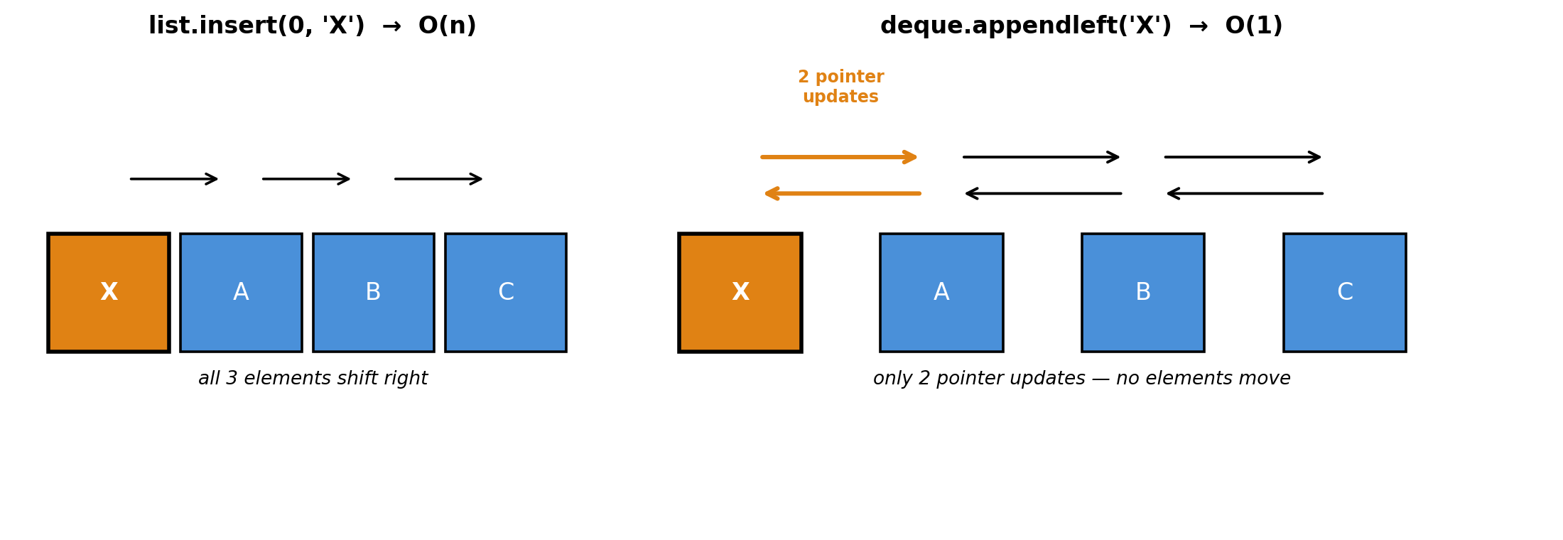
Left: inserting 'X' at the front of [A, B, C] forces all three elements to shift right. Right: deque rewires two pointers, so A, B, C don’t move.
Costs: appendleft/popleft/append/pop \(O(1)\) · index access \(O(n)\).
Use when: both ends are hot, like queues and double-ended buffers. Never list.pop(0) in a loop.
E. Hash map / set: both primitives combined
Why · \(O(1)\) average lookup, insert, delete. Replacing a list scan with a set lookup is the most common O(n²)→O(n) win in real code. Where · any time your first instinct is “scan a list for X”.
A hash table is built from both primitives: a contiguous array of \(m\) buckets, where each bucket is the head of a pointer-chained list of items that hash to the same slot.
The hash function \(h : \{0,\ldots,u-1\} \to \{0,\ldots,m-1\}\) maps a key to a bucket index. Instead of one slot per possible key (universe size \(u\)), we use only \(m \approx n\) slots.
Figure 7 · Hash table with chaining (\(m=8\) buckets, \(h(k) = k \bmod 8\)).
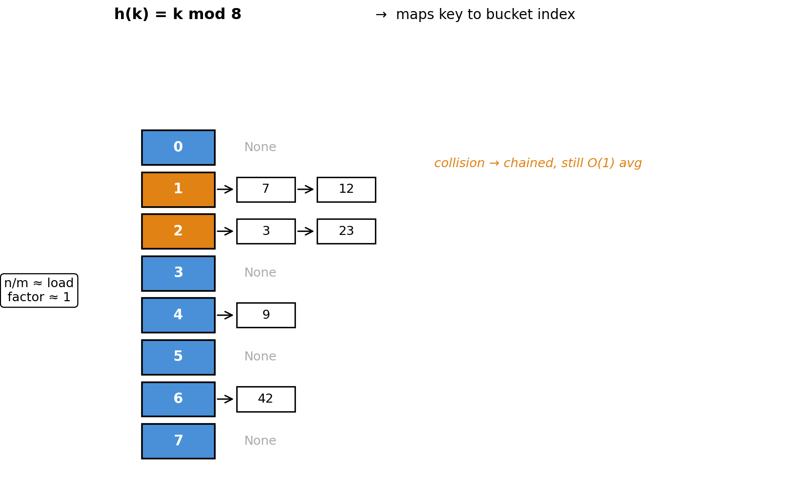
Orange buckets have collisions; their chains stay short (\(n/m \approx 1\)), so lookup is still \(O(1)\) average. The trace below uses \(m=5\) for simplicity: same principle, smaller numbers.
Mechanism trace: d[k] (lookup).
Table: \(m=5\), \(h(k)=k \bmod 5\). Stored keys: 2, 7, 14.
Since \(2\bmod5=2\), \(7\bmod5=2\), \(14\bmod5=4\):
table = [[], [], [2, 7], [], [14]], so bucket 2 has collision chain \([2 \to 7]\).
Look up d[7]:
- \(b = 7 \bmod 5 = 2\), one arithmetic op.
- Go to
table[2], chain \([2 \to 7]\). -
2 == 7? No. Advance.7 == 7? Yes → found. - Expected chain length \(= n/m = 3/5 < 1\) → \(O(1)\) expected.
- \(O(1)\) in practice: Python picks a random constant at startup and mixes it into every hash computation (the “hash seed”). This means an attacker cannot craft keys that all land in the same bucket, which is the only way to get O(n) chains in practice. The table also resizes when \(n/m > \text{threshold}\) (same amortized doubling as Section A), keeping chain length \(\approx 1\).
The four sub-uses (from the upcoming pattern-triggers post):
-
Membership:
x in s→ \(O(1)\). -
Dedup:
set(items)removes duplicates in \(O(n)\). -
Count:
Counter(items)gives frequency map in \(O(n)\). -
Group-by:
d.setdefault(key, []).append(val)buckets items by key in \(O(n)\).
Costs: lookup/insert/delete \(O(1)\) average · \(O(n)\) worst case (all keys collide) · no ordering.
The \(O(1)\) lookup is what eliminates the inner loop. Before vs after:
# Before: O(n²), inner scan on every outer step
for x in a:
    for y in b:
        if x == y: ...

# After: O(n), pre-load b into a set, one lookup per outer step
b_set = set(b)          # O(n) once
for x in a:             # O(n)
    if x in b_set:      # O(1)
        ...
Recognition trigger on the upcoming pattern-triggers post; PR-audit version on the upcoming DSA-at-work post.
🔗 Connections
- Memory and cost rules: Foundations.
- Master map: Overview.
- Linked-list idioms (reversal, Floyd’s cycle), two-pointer and window techniques: Array & String Techniques.
- Hash map as adjacency list in graphs; stack in DFS; deque in BFS: Graphs.
- Hash sub-uses (membership / dedup / count / group-by) as recognition triggers: the upcoming pattern-triggers post.