8. Transformer
⏮️ I recommend reading the RNN post first for the encoder-decoder architecture.
Transformer
In the last section we learned that RNNs have problems with learning
relations between the first parts of an input sequence with the output
and later parts of the input sequence. An architecture without this
structural problem is the transformer. The architecture was published by
Attention
Let us introduce this concept with an example. Figure 7 shows an encoder-decoder network with attention similar to the previous encoder-decoder RNN (Figure 6). The core idea of attention is defining the hidden state of the decoder-RNN as a function of every hidden state from the encoder-RNN for every time period without recursion. The result of the attention function is the context vector. We will use this vector for every output element. In the specific network in Figure 7, the context vector is a function of both the decoder states \(s\) and the encoder states \(h\). Further, it is additionally concatenated with \(s\) to predict the output layer.
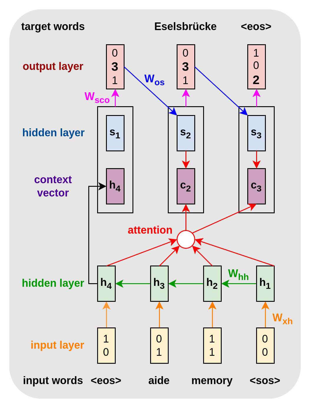
Figure 7. Encoder-Decoder with attention. In contrast to the encoder-decoder RNN, the output layer is a function of the concatenation of the hidden states and a time-dependent context vector (black boxes). The main idea is that the context vector \(c_t\) is a function of all hidden states \(\{h_t\}_{t=1}^{T}\) instead of only the last one (and the previous state \(s_{t-1}\)). This function is called attention (red). The black box represents vector concatenation. \(c_1\) is initialized with $h_4$, \(s_1\) with arbitrary values, and \(o_1\) is discarded.
The attention function that returns the context vector for output \(y_t\) wit attention scores for each input is given by the following expression:
\[\begin{align}c_t = \sum_{i=1}^n \alpha_{t,i} h_i\end{align}\]\(\alpha_{t,i}\) is a softmax function of another function score that measures how well output \(y_t\) and input \(x_i\) are aligned through the encoder state \(h_i\):
\[\begin{align}\alpha_{t,i} = \text{align}(y_t,x_i) = \frac{\exp \text{score}(s_{t-1}, h_i)}{\sum_{j=1}^n\exp\text{score} (s_{t-1}, h_j)}.\end{align}\]There are many different scoring functions
Another option for an encoder-decoder with attention is using a self-attention mechanism to compute the context vector, for example, with score \((h_j, h_i)=\frac{h_j^T h_i}{\sqrt{d}}\). We can use the scores, for instance, in machine translation, to model how important the previous words are for translating the current word in a sentence. Note that we can execute many of these operations in parallel for the whole input and output sequences using matrix operations.
Next, we will discuss an expansion of the attention mechanism and how it is applied to the transformer’s encoder and decoder, separately. Finally, we will look at the complete model, and how it replaces the positional information from the encoder RNN in a simple way without any recurrence.
Key, Value and Query
As we do not use recurrence of single sequence elements anymore, let us denote the whole sequence of input embeddings by \(X \in \mathbb{R}^{L \times D^{(x)}}\). \(L\) can either be the complete input length \(T_x\) or later only a fraction of it. \(D^{(x)}\) is the input embedding’s length. Let us denote the sequence of output embeddings by \(Y \in \mathbb{R}^{M \times D^{(y)}}\). The transformer uses an extension of the attention mechanism, the multi-head attention, as its core building block. The first step is that, instead of using the softmax of the scaled dot-product between encoder states \(h\) and decoder states \(s\) directly as in the last section, it uses the scaled dot-product with two different input encodings, \(K=XW^k \in \mathbb{R}^{L \times D_k}\) and \(V=XW^v \in \mathbb{R}^{L \times D_v}\), and an output encoding \(Q=YW^q \in \mathbb{R}^{M \times D_k}\), with \(W^k \in \mathbb{R}^{D^{(x)} \times D_k}, W^q \in \mathbb{R}^{D^{(y)} \times D_k}\) and \(W^v \in \mathbb{R}^{D^{(x)} \times D_v}\). Note that source and target embeddings are projected into a shared or common vector space with consistent dimensions. With that, we can compute the dot product between input and output sequences of different fixes maximal length and obtain \(D_v\) embeddings of dimension \(M\). We compute attention with
\[\begin{align}c(Q,K,V)=\text{Softmax}\big(\frac{QK^T}{\sqrt{n}}\big)V.\end{align}\]In this equation, we refer to \((K, V)\) as key-value pairs, and \(Q\) as the query (see Appendix for an explanation of the names). By interpreting the dot product as a similarity measure, the context matrix \(c(Q,K,V) \in \mathbb{R}^{M \times D_v}\) illustrates the similarity between the input and a representation of the input, which is weighted by its similarity to the output (in the context of cross-attention).
Let’s summarize the computation in simpler terms: The context matrix comprises \(M\) rows, one for each output element, and \(D_v\) columns, corresponding to the dimensions of the value vectors. To delve deeper, we consider each row in the resulting context matrix \(c(Q, K, V)\). For a specific output element, its row is computed by taking a weighted sum of the value vectors from matrix \(V\). These weights are determined by the similarity between the query vector for that output element (from matrix \(Q\)) and the key vectors for all elements in the input sequence (from matrix \(K\)). The Softmax function is applied to normalize these weights for each output element.
Importantly, we apply masking to the embeddings for unseen target elements at each time step, ensuring that only relevant input elements contribute to the computation. The context matrix serves as the foundation for subsequent computations in the attention mechanism, allowing the model to determine how much attention to allocate to each part of the input sequence when generating the output.
In the transformer encoder, there is an important module where the queries are also source representations and in the decoder, there is a module where keys and values are also target representations (self-attention).
Multi-Head Attention
Instead of computing the attention once, the multi-head approach splits the three input matrices into smaller parts and then computes the scaled dot-product attention for each part in parallel. The independent attention outputs are then concatenated and linearly transformed into the next layer’s input dimension. This allows us to learn from different representations of the current information simultaneously with high efficiency. In the CNN post, we have already introduced the principle of applying the same operation multiple times with different learned sets of parameters: remember that CNNs contain stacks of multiple filters to provide the model with multiple feature maps, each covering different aspects of the input image. Multi-head attenttion is defined by
\[\begin{align}\text{MultiHead}(X_q, X_k, X_v)= [ \text{head}_1;...;\text{head}_h ] W^o,\end{align}\]where \(\text{head}_i=\)Attention\((X_q W^q_i, X_k W^k_i, X_v W^v_i)\) and \(W_i^q \in \mathbb{R}^{D^{(y)} \times D_v /H}\), \(W_i^k \in \mathbb{R}^{D^{(x)} \times D_k / H}\), \(W_i^v \in \mathbb{R}^{D^{(x)} \times D_v /H}\) are matrices to map input embeddings of chunk size \(L \times D\) into query, key and value matrices. \(W^o \in \mathbb{R}^{D_v \times D}\) is the linear transformation in the output dimensions. These four weight matrices are learned during training. Target self-attention and cross attention layers compute outputs in \(\mathbb{R}^{M \times D}\), and source self-attention calculates outputs in \(\mathbb{R}^{L \times D}\).
Transformer Encoder
The Transformer architecture, as introduced by Vaswani et al. in 2017
Figure 8. Transformer encoder. The Transformer Encoder consists of a stack of identical layers, including a multi-head self-attention layer (Red) for capturing contextual information and a position-wise fully-connected feed-forward network for introducing non-linearity. These two components work synergistically to process input sequences effectively and extract meaningful representations, with attention parameters focusing on dependencies and position-wise FNN parameters capturing position-specific patterns. Image source:
In its original form, the encoder consists of a stack of N = 6 identical layers, each with unique parameters. These layers consist of two critical components:
-
Multi-head self-attention layer (red): This layer is the cornerstone of the Transformer’s ability to capture contextual information from input sequences. It allows the model to focus on different parts of the input sequence simultaneously. Self-attention is a mechanism where each input element contributes to the representation of every other element, making it robust to capturing long-range dependencies and essential for tasks such as machine translation
. -
Position-wise fully-connected feed-forward network (blue): This layer introduces non-linearity into the network, allowing the model to capture complex patterns and relationships within the data.
These two components, self-attention and position-wise FNN, are fundamental in processing input sequences of varying length effectively and extracting meaningful representations. It is crucial to understand the clear distinction between the parameters used in the attention mechanism and those employed in the position-wise fully-connected feed-forward network (FNN) in order to understand the modules specific tasks, mechanisms and how they can process sequences of varying length:
-
Attention parameters: The attention mechanism, which consists of the attention parameters, is responsible for capturing dependencies and relationships between elements within the input sequence. It does this by assigning different attention weights to each element in the sequence based on its relevance to other elements. This allows the model to focus more on important elements and less on irrelevant ones. Importantly, the attention mechanism can adapt to input sequences of different lengths because the attention weights are calculated dynamically for each position in the sequence. Longer sequences may receive different attention distributions compared to shorter sequences.
-
Position-wise FNN parameters: The position-wise FNN introduces non-linearity and complexity into the model. While the same position-wise FNN is applied to each position within the input sequence independently, the transformations performed by this network can capture position-specific patterns and relationships. This means that even though the same FNN parameters are shared across positions, the content of the positions can lead to different activations and outputs, allowing the model to handle sequences of varying lengths. The majority of the model’s parameters are part of this module.
The combination of attention and position-wise FNN parameters enables the transformer to process input sequences of different lengths by dynamically adjusting the attention weights and capturing position-specific information. The attention mechanism provides a mechanism for the model to focus on relevant parts of the sequence, while the position-wise FNN allows for nonlinear transformations that can adapt to different content in the sequence. This flexibility is one of the key strengths of the Transformer architecture and makes it well-suited for a wide range of natural language processing tasks where input sequences may vary in length.
Transformer Decoder
The decoder network, illustrated in Figure 9, is equally crucial in the Transformer architecture, as it enables the generation of sequences autoregressively based on the encoded source representation.
Figure 9. Transformer decoder. The Transformer decoder plays a crucial role in autoregressively generating sequences based on encoded source representations. It includes a masked multi-head self-attention layer to capture dependencies within the target sequence, a multi-head cross-attention layer for accessing relevant source information, and a fully-connected feed-forward network to model complex relationships, all followed by normalized residual layers for stability. Image source
Similar to the encoder, the decoder comprises N = 6 identical layers. These layers consist of:
-
Masked Multi-Head Self-Attention Layer (Red): In the decoder, this layer is masked to prevent attending to future positions in the output sequence. It focuses on capturing dependencies among elements within the target sequence that have already been generated. This masking is crucial for ensuring the autoregressive nature of the decoder, allowing it to generate sequences one element at a time
. Specifically, the masked multi-head self-attention layer in the decoder prevents the model from attending to future positions in the (Shifted) Outputs sequence. This mechanism ensures that each position in the (Shifted) Outputs sequence is generated based on the previously generated elements, adhering to the autoregressive nature of sequence generation. -
Multi-Head Cross-Attention Layer (Red): The decoder generates queries from the previously generated target representations and uses them to attend to the encoded source representations. This mechanism ensures that the decoder accesses relevant information from the source to generate the next part of the target sequence.
-
Fully-Connected Feed-Forward Network (Blue): Similar to the encoder, this layer introduces non-linearity, enabling the decoder to model complex relationships.
Each of these layers is followed by a normalized residual layer (yellow), contributing to the stability and effectiveness of the Transformer’s decoding process.
The Complete Transformer Architecture
Figure 10 presents the complete Transformer architecture:
Figure 10. The complete transformer. In its original form, the Transformer processes both source and target sequences through embedding layers (light blue), creating representations of dimension D = 512 for each element. Adding sinusoidal positional encoding vectors to the embeddings pallows the model to distinguish between different positions and capture positional dependencies. The Transformer’s ability to handle input and output sequences of different lengths is primarily achieved through its masking mechanism. Padding masks ensure that the model does not consider padded elements when calculating attention scores, and the self-attention mechanism can adapt to variable-length sequences while maintaining coherence. The term “(Shifted) Outputs” emphasizes the autoregressive nature of the decoding process, where each output position depends on previously generated positions. Image source
The Transformer possesses several critical properties:
-
Inductive Bias for Self-Similarity: The self-attention mechanism empowers the model to identify recurring patterns or themes within the data, irrespective of their positions. This inductive bias is invaluable in real-world domains where recurrence is a prevalent pattern
. -
Expressive Forward Pass: The Transformer establishes direct and intricate connections between all input and output elements, facilitating the learning of complex algorithms in a few steps.
-
Wide and Shallow Compute Graph: Thanks to residual layers and matrix products in attention layers, the compute graph remains wide and shallow. This promotes fast forward and backward passes on parallel hardware while mitigating issues like vanishing or exploding gradients through techniques such as layer normalization and dot product scaling.
Complexity Comparison
To conclude this chapter, let’s compare the complexities of the three main architectures in deep learning, as shown in Table 2, based on the survey by Lin et al. in 2022
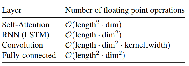
Table 2. Comparison of computation complexity between models. The “length” refers to the number of elements in the input sequence, and “dim” denotes the embedding depth for each element. It’s worth noting that attention mechanisms, as used in Transformers, excel when the input sequence length is much smaller than the embedding depth. This advantage is evident in tasks like machine translation or question-answering, where capturing long-range dependencies is crucial. However, for direct application to image data, which inherently has a larger input length (e.g., CIFAR images with 3072 elements), preprocessing steps are necessary to reduce the input length effectively.
In summary, the Transformer architecture’s success lies in its ability to capture complex dependencies, handle sequences of varying lengths, and process them efficiently through its innovative components, making it a fundamental building block in modern deep learning.
Appendix — Naming Convention of Key, Value and Query
The naming convention of “key,” “query,” and “value” in the context of attention mechanisms is rooted in their respective roles and functions within the mechanism. These names help clarify how each component contributes to the computation of the context vector in attention.
Key (K): The key is essentially a set of representations derived from the input sequence (or encoder states in the case of sequence-to-sequence models like the Transformer). These representations are crucial for determining how much attention should be given to each element in the input sequence when generating an output. Keys are used to match against the queries.
Reasoning: Think of the “key” as a guide or a set of pointers that specify which parts of the input sequence are relevant for generating the output. It helps the model identify what to focus on.
Query (Q): The query represents what the model is currently trying to generate or pay attention to within the output sequence. In other words, it’s a representation of the current target or decoder state.
Reasoning: The “query” represents the current “question” or “target” that the model is interested in. It’s used to determine how well each element in the input sequence (represented by keys) aligns or matches with the current target.
Value (V): The value component contains the information that will be used to produce the context vector. Like keys, values are derived from the input sequence. However, they represent the content or information associated with each element in the input sequence.
Reasoning: The “value” carries the actual information that the model will use when generating the output. It’s like the “answer” or “content” associated with each part of the input sequence.
To put it all together, the attention mechanism calculates a weighted sum of values based on the similarity between the query and keys. This weighted sum, known as the context vector, is used to determine how much each part of the input sequence should contribute to the current output. The keys help identify which parts are relevant, the query specifies what is being looked for, and the values provide the information to be used.
This naming convention, while abstract, makes the roles and relationships of these components intuitive, facilitating a clearer understanding of how attention mechanisms work in neural networks.
Citation
In case you like this series, cite it with:
@misc{stenzel2023deeplearning,
  title   = "Deep Learning Series",
  author  = "Stenzel, Tobias",
  year    = "2023",
  url     = "https://www.tobiasstenzel.com/blog/2023/dl-overview/
}