Trackformer — Multi-Object Tracking with Transformers
A lower-level explanation of the paper Multi-Object Tracking with Transformers (Meinhardt et al., 2022) including DETR (Carion et al., 2020) and Deformable DETR (Zhu et al., 2020). 🎥
1.) Introduction
This blog post provides a detailed explanation of the transformer-based tracking model Trackformer
Multi-object tracking (MOT) is an important task in the Computer Vision domain. MOT is closely related to object detection because tracking models utilize the detections in each frame of a video with the aim of assigning the same ID to the same objects across different frames over time. Trackformer uses the transformer-based object detector DEtection TRansformer (DETR)
We will delve into both models in more detail separately. First, we will explore DETR
2.) DETR as Object Detector
Previous object detection systems incorporate various manually designed
elements, such as anchor generation, rule-based training target
assignment, and non-maximum suppression (NMS) post-processing
Complete transformer-based DETR architecture
The overall model has
three components as depicted by Figure
1. The first component is a conventional
CNN backbone that generates a lower-resolution activation map many
channels. The transformation from large embedding length (image height
\(\cdot\) width) to large embedding depth is crucial for the efficiency of
the attention modules (see
Table 2. The second component is the transformer
encoder-decoder. In contrast to the original decoder by
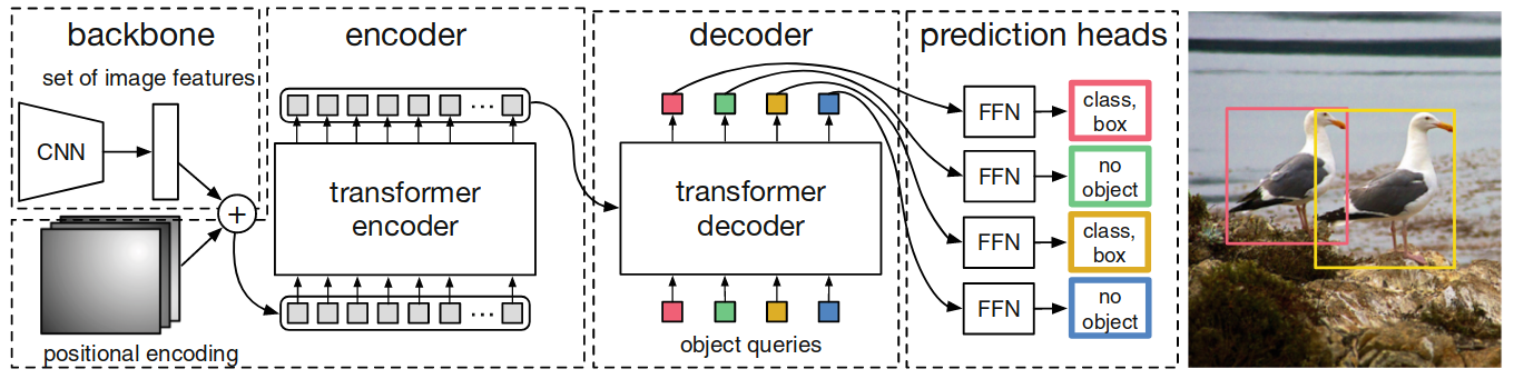
Figure 1. High-level DETR architecture with CNN backbone,
transformer-encoder decoder and FFN prediction heads. In contrast to the
autoregressive sequence generation in
The transformer allows the model to use self- and cross-attention over the object queries to include the information about all potential objects with pair-wise relations in their prediction of only one potential object, while using the whole image as context.
Object Detection Set Prediction Loss
During training, we want to
learn predictions that have the right number of no classes and the right
number of classes with the right class label and bounding box. Formally,
we achieve this the following way: From the transformer decoder
prediction head, DETR infers \(N\) predictions for the tuples of bounding
box coordinates and the object class. \(N\) has to be at least as large as
the maximal number of objects on one image. The first tuple element are
the bounding box coordinates, denoted by \(b \in [0,1]^4\). These are four
values: the image-size normalized center coordinates, and the normalized
height and width of the box w.r.t. the input image’s borders. Using
center coordinates and normalization help us to deal with images of
different sizes. Examples for the second tuple element, class \(c\), are
"person A", for person detection, or "car" for object detection. The
remaining class is the "no object" class, denoted by \(\emptyset\). For
every image, we pad the target class vector \(c\) of length \(N\) with
\(\emptyset\) if the image contains less than \(N\) objects. To score
predicted tuples
\(\hat{y}=\{\hat{y}_i\}_{i=1}^N=\{(\hat{c}_i,\hat{b}_i)\}_{i=1}^N\) with
respect to the targets \(y\),
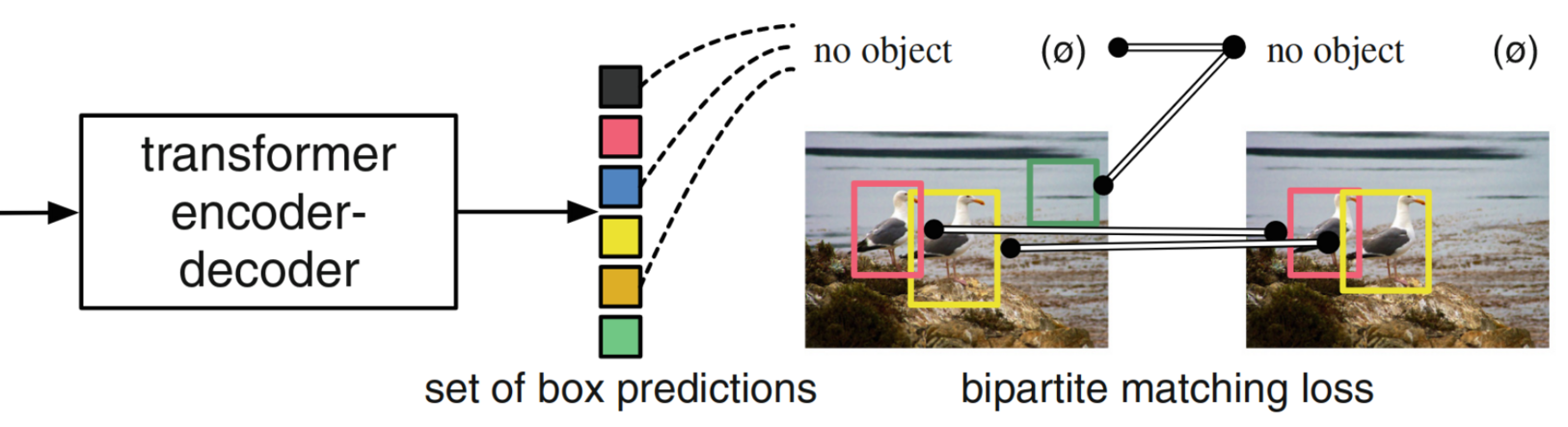
Figure 2. DETR training pipeline with bipartite matching loss. The
loss function generates an optimal one-to-one mapping between
predictions and targets according to bounding box and object class
similarity (colors). In this unique permutation of N classes, class predictions with no
match among the class targets are regarded as “no object” predictions,
too (green). Image source:
The next section describes the loss function required for the bipartite matching between predicted and target detections that is optimal in terms of bounding box and class similarity. We find the optimal permutation of predicted detections \(\hat{\sigma}\in\mathcal{\mathfrak{S}}_N\) of \(N\) elements from:
\[\begin{align} \hat{\sigma} = arg\,min_{\sigma\in\mathcal{\mathfrak{S}}_N} \sum_{i}^{N} \text{L}_{\text{match}}(y_i, \hat{y}_{\sigma(i)}), \end{align}\]where \(\text{L}_{\text{match}}\) is a pair-wise matching cost between
target \(y_i\) and prediction \(\hat{y}\) with index \(\sigma(i)\). We compute
the assignment efficiently with the Hungarian matching algorithm
We want to assign predictions and targets that are close in terms of class and bounding box. Thus, the matching considers both the class score for every target and the similarity of predicted and target box coordinates. We reward a high class score for the target class and a small bounding box discrepancy. To this end, let us denote the index function by \(\text{I}\), the probability of predicting class \(c_i\) for detection with permutation index \(\sigma(i)\) by \(\hat{p}_{\sigma(i)}(c_i)\) and the predicted box by \(\hat{b}_{\sigma(i)}\). With that, we define the pair-wise matching loss as
\[\begin{align} \text{L}_{\text{match}}(y_i, \hat{y}_{\sigma(i)}) = -\text{I}_{c_i\neq\emptyset} \hat{p}_{\sigma (i)}(c_i) + \text{I}_{c_i\neq\emptyset} \text{L}_{\text{box}}(b_{i}, \hat{b}_{\sigma(i)}). \end{align}\]Here, our objective is to find the best matching for the "real" classes \(c \neq \emptyset\) by ignoring class predictions that are directly mapped to "no class" by the prediction. However, the model still has to learn not to predict too many real classes. Given our optimal matching \(\hat{\sigma}\), we achieve this by minimizing the Hungarian loss. The function is given by
\[\begin{align}\text{L}_{\text{Hungarian}}(y, \hat{y}) = \sum_{i=1}^N \left[-\log \hat{p}_{\hat{\sigma}(i)}(c_{i}) + \text{I}_{c_i\neq\emptyset} \text{L}_{\text{box}}\Big(b_{i}, \hat{b}_{\hat{\sigma}}(i)\Big)\right]\end{align}\]The difference to the matching loss is two-fold. First, we now penalize wrong assignments to all classes including "no class" with the first class-specific term. We do not include the "no class" instances to the box loss \(\text{L}_{\text{box}}\) because they are not matched to a bounding box anyway. Second, we scale the class importance compared to the bounding boxes by taking the log of predicted class probabilities. In practice, the class term is further reduced for "no class" objects to take class imbalance into account. The last expression is the box loss. It is the L1 loss of the bounding box vector \(b_i\). Note, however, that the L1 loss penalizes larger boxes. The following equations shows the expression:
\[\begin{align} \text{L}_{\text{box}}(b_{i}, \hat{b}_{\sigma(i)}) = \lambda_{\text{box}}||b_{i}- \hat{b}_{\sigma(i)}||_1, \end{align}\]where \(\lambda_{\text{box}} \in \mathbb{R}\) is a hyperparameter. We normalize the loss by the number of objects in each image.
DETR’s drawbacks
In spite of its intriguing design and commendable
performance, DETR encounters certain challenges. Firstly, it requires
significantly more training epochs to reach convergence compared to
existing object detectors. For instance, when evaluated on the COCO
benchmark
3.) Trackformer as Multi-Object Tracker
Trackformer
With the described approach, we train the model to not only decode learned object queries into representations that can detect objects but also to use the decoded queries again as decoder input to detect the same object when possible. If we match the decoder output from an object query in frame \(t-1\), it is re-used as an additional track query as decoder input for frame \(t\). If its output is matched again, we assume that both detections belong to the same object with ID \(k\).
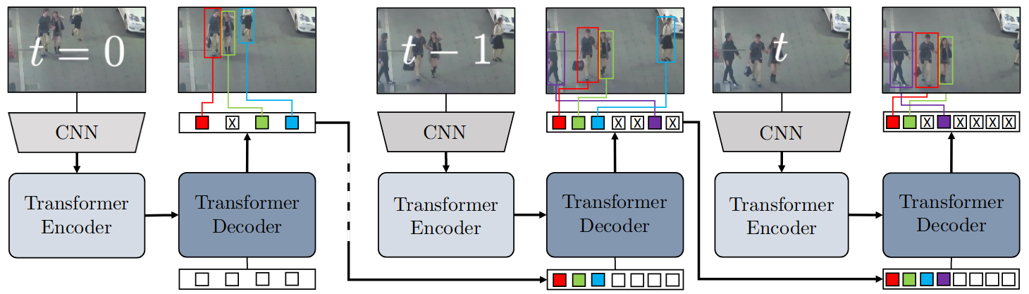
Figure 3.Trackformer architecture. Trackformer extends DETR to
tracking on video data by feeding the decoded object queries that are
matched to actual objects as additional autoregressive tracking
queries (colored detection squares) next to the object queries for
the next image into the transformer decoder (dark blue). The decoder
processes the set of Ntrack + Nobject
queries to further track or remove existing tracks (light blue) and to
initialize new tracks (purple). Image source:
Set prediction loss
We now want to formulate a loss that allows the model to learn the bipartite matching \(j=\pi (i)\) between target objects \(y_i\) to the set of both object and track query predictions \(\hat{y}_j\). For this purpose, let us denote the subset of target track identities at frame \(t\) with \(K_t \subset K\). This is different from DETR as \(K\) contains all object identities for all images in the video sequence. These object or track identities can be present in multiple frames, i.e. they can intersect from frame to frame. Trackformer takes three steps to associate queries with targets. The last step corresponds to DETR’s method. The steps to obtain the mapping of predicted detections to target detections \(\hat{\sigma}\) for one frame are the following: first, we match \(K_{\text{track}} = K_{t-1} \cap K_t\) (target objects in the current frame that were also present in the previous frame) by track identity. This means, we associate these targets with the output from the previous query. Second, we match \(K_{\text{leaving}} = K_{t-1} \setminus K_t\) (objects leaving the scene between two frames) with background class \(\emptyset\). And third, we match \(K_{\text{init}} = K_{t} \setminus K_{t-1}\) (objects entering the scene) with the \(N_{\text{object}}\) object queries by minimum cost mapping based on object class and bounding box similarity the same ways as DETR assigned its targets to object queries.
Output embeddings which were not matched, i.e. 1) proposals with worse class and bounding box similarity than others or 2) track queries without corresponding ground truth object, are assigned to background class \(\emptyset\).
With this order, we prioritize matching track queries from the last frame even if object queries from the current frame yield more similar bounding boxes and classes. This is necessary because, in order to assign the same object ID to detections in multiple frames, we have to train the object queries to not only initialize a track after on pass through the decoder but also to detect the same object after two passes through the decoder with given the respective interactions from the image encodings.
The final set prediction loss for one frame is computed over all \(N=N_{\text{object}}+N_{\text{track}}\) model outputs. Because \(K_{t-1} \setminus K_t\) (objects that left the scene) are not contained in the current-frame permutation, we write the loss as
\(\begin{align} \text{L}_{\text{MOT}}(y,\hat{y},\pi)=\sum_{i=1}^N \text{L}_{\text{query}}(y,\hat{y},\pi). \end{align}\) Further, we define the loss per query and differentiate two categories. First, we have the object query loss \(L_0\) for outputs from unmatched embeddings. And second, we have the track query loss \(L_1\) for outputs from matched embeddings that will be overtaken to the next time period as track queries. Formally, the query loss is given by
\[\begin{align}\text{L}_{\text{query}}= \begin{cases} \phantom{.}L_0 &= -\lambda_{\text{cls}} \log \hat{p}_i (\emptyset) \quad \phantom{..................}\text{if } i \notin \pi \\ \phantom{.}L_1 &= -\lambda_{\text{cls}} \log \hat{p}_i (c_{\pi=i}) + \text{L}_{\text{box}}(b_{\pi=i},\hat{b}_i) \quad \text{if } i \in \pi. \end{cases}\end{align}\]The expression captures two features: first, \(L_1\) rewards track queries that find the right bounding box for objects that are still present on the current frame and it rewards object queries with similar outputs to new objects. Second, \(L_0\) not only rewards track queries that predict the background class if their object has left the scene but also object queries that predict the background class if their bounding box prediction is off. The discussed details about track and object queries, and the matching rules with examples for assigned bounding boxes and losses are depicted in 4.
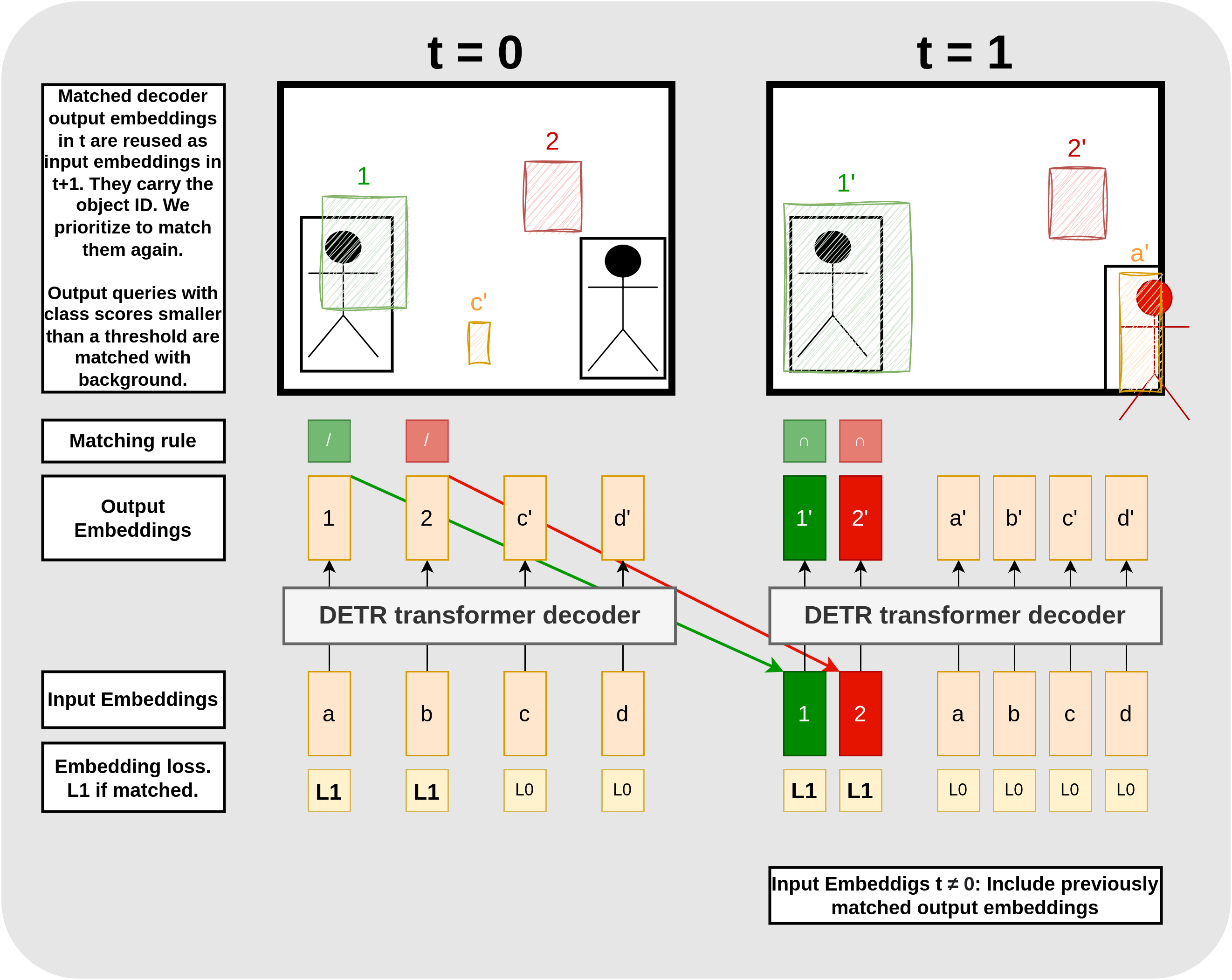
Figure 4. Training track and object queries. The black boxes are ground truth detections and the colorful, annotated boxes are predictions from the respective output embedding. Embeddings that do not spawn a box predict a class score smaller than the threshold. In t=0, the most similar boxes (green and red) are matched with the two target boxes according to matching step 2: Kinit (symbolized by “/”). For these boxes, we compute L1 based on boxes and class scores, and for the unmatched boxes, we compute L0 solely based on the class scores. Then we update the model parameters accordingly. The matched output embeddings are taken over as additional input embeddings, carrying the object IDs from the objects on the previous image. They are matched with priority according to matching step 1: Ktrack (symbolized by “∩”). Embedding 2’ is matched although the bounding boxes from output embedding a′ is more similar to the target. We feed embeddings 1′ and 2′ to the decoder in period t = 2 (see Figure 5).
Track query re-identification
What happens if objects are occluded or re-enter the scene? To deal with such cases, we keep feeding previously removed track queries for a patience window of \(T_{track-reid}\) frames into the decoder. During this window, predictions from track ids are only considered if a classification score higher than \(\sigma_{track-reid}\) is reached.
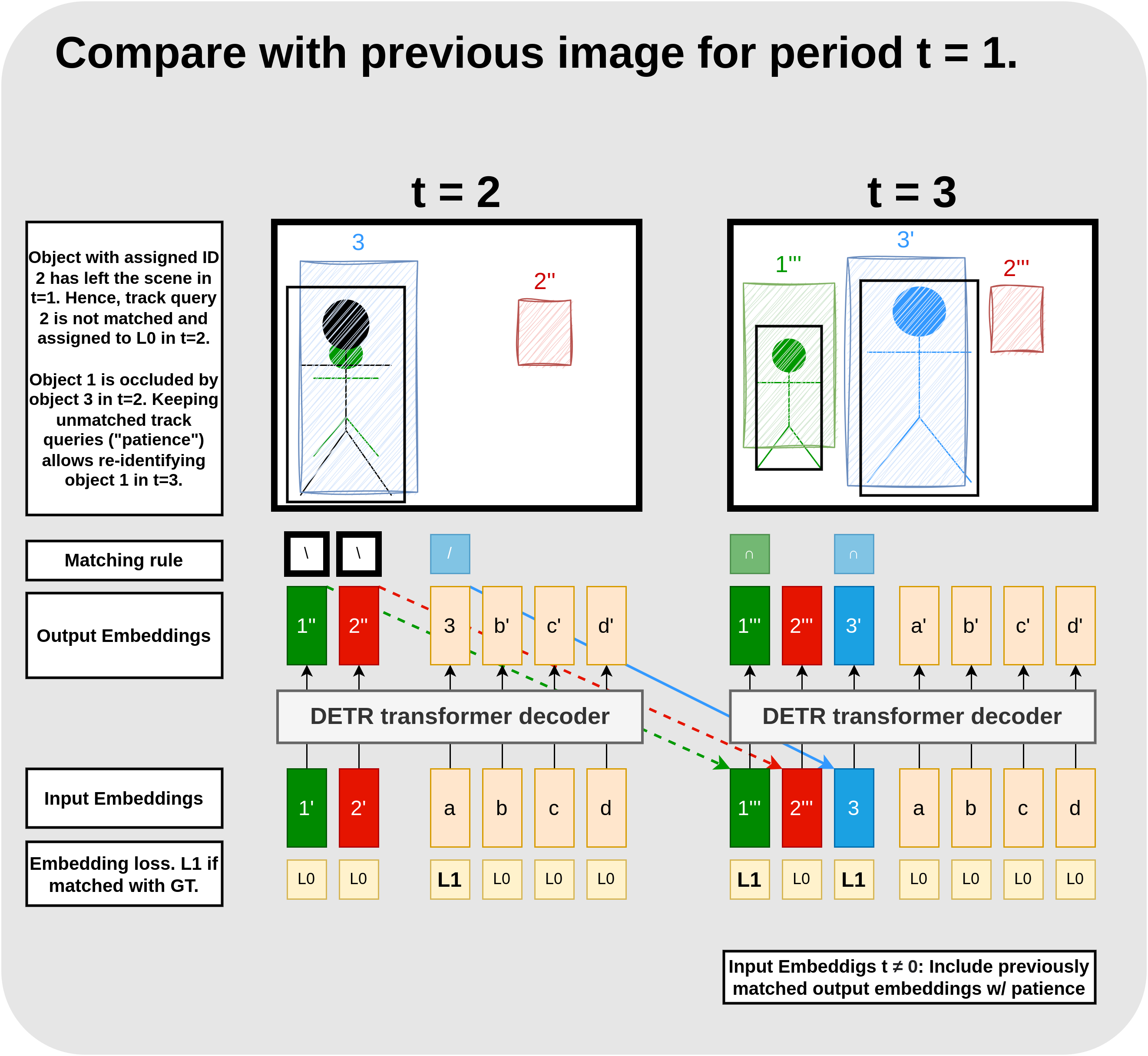
Figure 5. Training track queries with re-identification. Make sure to compare this Figure to Figure 4. From t = 1, we additionally feed output embeddings 1′ and 2′, carrying the object identities for pedestrian 1 (green) and pedestrian 2 (blue) to the encoder. However, pedestrian 2 has left the scene between t = 1 and t = 2 and pedestrian 1 is occluded by a news pedestrian with ID 3. Here, we depict the case where we have no ground truth annotation for the occluded pedestrian. Note that the prediction from embedding 1′ is quite reasonable given that pedestrian 1 is almost invisible. In contrast, embedding 2′ keeps predicting a bounding box in the close to the upper right corner independent of the image. Since there are no detections with IDs previously matched to 1 or 2, we cannot apply matching step 1: Ktrack (symbolized by “∩”) to output embeddings 1″ and 2″. Instead, we match both outputs with the background class according to step 2 Kleaving (symbolized by “∖”). Assuming the green pedestrian would be annotated, however, we would have apply step 1: Ktrack (symbolized by “∩”) to embedding 1″ instead. To track the new pedestrian with ID 3, we apply matching step 3: Kinit (symbolized by “/”) to embedding 3 and update the model according to the respective losses. Since we keep unmatched embeddings with patience, we take over embeddings 1″ and 2″ to the next frame in addition to embedding 3. This allows the model to re-identify object 1 (green) in period t = 3.
Results
Trackformer achieved state-of-the-art performance in
multi-object tracking on MOT17 and MOT20 datasets. It is important to pre-train the model on large tracking datasets, to use track augmentations, and probably also to use pre-trained detection weights for tracking-specific pre-training.
4.) Extra. Deformable DETR as More Efficient Detector
In order to address DETR’s disadvantages,
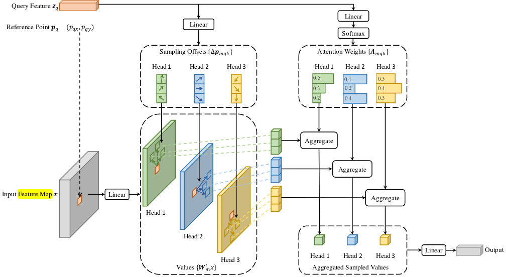
Figure 6. High-level Deformable DETR architecture. We extract three
feature maps at different resolution levels from the CNN backbone. In
the encoder, we aggregate the information from all multi-scale feature
maps with deformable self-attention, attending only to a learned sample
of important locations around a learned reference point from every
feature map for each feature map (deformable attention). This results in
three encoder feature maps of the same dimensions. In the decoder, the
learned object queries extract features from queries and values from
themselves with conventional self-attention and from the keys from the
encoder feature maps with deformable cross-attention. Again, for each
object query, the learned reference point and a set of learned offsets
is used to only query a set of keys from the encoder. With that, we
replace the self-attention modules in the encoder and the and
cross-attention modules in the decoder with 4 heads of the deformable
attention module and learn from feature maps at different resolutions.
This makes the transformer’s complexity as a function of pixel number
sub-quadratic and allows the model to better learn objects at strongly
distinct scales. Image source:
Multi-Head Attention Revisited
When provided with a query element (e.g., a target word in the output sentence) and a set of key elements (e.g., source words in the input sentence), the multi-head attention module aggregates the key contents based on attention weights, which gauge the compatibility of query-key pairs. In order to enable the model to focus on diverse representation subspaces and positions, the outputs of various attention heads are combined linearly using adjustable weights.
Let \(q \in \Omega_q\) denote an index for the query element represented by feature \(z_q \in \mathbb{R}^C\), and let \(k \in \Omega_k\) denote an index for the key element represented by feature \(x_k \in \mathbb{R}^C\) with feature dimension \(C\) and set of query and key elements \(\Omega_q\) and \(\Omega_k\), respectively. We compute the multi-head attention feature for query index \(q\) with
\[\begin{align}\text{MultiHeadAttn}(z_q, x) = \sum_{m=1}^M W_m [\sum_{k \in \Omega_k} A_{mqk} \cdot W_m^{T} x_k],\end{align}\]where \(m\) is index the attention head and \(W_m \in \mathbb{R}^{C \times C_v}\) are learned weights with \(C_v = C/M\). We normalize the attention weights \(A_{mqk} \propto \text{exp}\{\frac{z_q^T U_m^T V_m x_k}{\sqrt{C_v}}\}\) with learned weights \(U_m, V_m \in \mathbb{R}^{C \times C_v}\) to \(\sum_{k \in \Omega_k} A_{mqk}=1\). In order to clarify distinct spatial positions, the representation features, denoted as \(z_q\) and \(x_k\), are formed by concatenating or summing the element contents with positional embeddings.
Deformable Attention
The main challenge in applying Transformer
attention to image feature maps is that it considers all potential
spatial locations. To overcome this limitation,
where \(k\) indexed the sampled keys and \(K \ll HW\) is the total number of sampled keys. Futher, \(\Delta p_{mqk} \in \mathbb{R}^2\) denotes the sampling offset and \(A_{mkq}\) the attention weights of the \(k^{\text{th}}\) sampling point in the \(m^{\text{th}}\) attention head, respectively. The attention weights are normalized to own over the sample keys. We feed query feature \(z_q\) to a \(3MK\)-channel linear projection operator. The inital \(2MK\) channels encode the sampling offsets \(Delta p_{mkq}\), and the latter \(MK\) channels are used as input to the softmax function to compute the attention weights \(A_mqk\).
Multi-scale Deformable Attention
We extend the deformable attention module to multiple differently-scaled feature maps with a few small changes. Let \(\{x^l\}_{l=1}^L\) denote the set of differently scaled feature maps, where \(x^l \in \mathbb{R}^{C \times H_l \times W_l}\) and let \(\hat{p}_q \in [0,1]^2\) denote the normalized reference points for each query element element \(q\). Then, we calculate the multi-scale deformable attention with
\[\begin{gathered} \text{MSDeformAttn}(z_q, \hat{p}_q, \{x^l\}_{l=1}^L) = \\ \sum_{m=1}^M W_m [\sum_{l=1}^L \sum_{k \in \Omega_k} A_{mlqk} \cdot W_m^{T} x^l (\phi_l (\hat{p}_q ) + \Delta p_{mlqk})], \end{gathered}\]where \(l\) indexes the input feature and we expand the normalized attention weights and the reference point by this dimension. \(\hat{p}_q \in [0,1]^2\) are also normalized coordinates with \((0,0)\) and \((1,1)\) as top-left and bottom-right coordinates, respectively. Function \(\phi_l(\hat{p}_q )\) is the inverse of the normalization function and maps \(\hat{p}_q\) back to the respective feature map coordinates. In constrast to the singlescale deformable attention module, we sample \(LK\) feature map points instead of \(K\) points and interact the different feature maps with each other.
Results
On the COCO benchmark for object detection, Deformable DETR outperforms DETR, particularly in detecting small objects, while requiring only about one-tenth of the training epochs.