⏮ 5. Feedforward Neural Networks 7. Recurrent Neural Networks ⏭

6. Convolutional Neural Networks

🔑️ Key sections about parameter sharing, inductive biases, skip connections, and cross-correlation.

2023 · dl-fundamentals neural-net-archetype backprop cross-correlation inductive-bias receptive-field compute-graph

Convolutional Neural Networks

A Convolutional Neural Networks (CNN) is type of neural network architecture that is specifically designed for input data where the tabular arrangement includes a spatial meaning. Moreover, the features of one example are not stored in a vector of different property values but \(x\) is a multi-dimensional array (i.e. a tensor). For instance, the data for a color image could have dimensions \(32 \times 32 \times 3\). The first two dimensions represent the height and the width of the pixels and the third dimension stands for three color channels red, green and blue. We can find these spatial relationships in many data, not only in images. Further examples are sound spectrogram or sentence data. The main motivation for CNNs is to reduce the complexity with parameter sharing by focusing on relations between spatially close data points.

Cross-correlation

The core building block of a CNN is the Convolutional Layer (or CONV layer). The main operation in this layer is the cross-product between tensors. We denote the cross-product between two tensors \(I\) and \(W\) as \(I \star W = O\). \(I\) is the input and \(W\) is the kernel or the filter. If the two matrices are three dimensional tensors, then the third dimension of both tensors must have equal length. Let \(i_1, i_2\) and \(f_1, f_2\) be the width and the height of the input and the filter, respectively. The output, activation map O, has dimension \((i_1 - f_1 + 1) \times (i_2 - f_2 + 1)\). Accordingly, the cross-product for one output element is given by the following formula :

\[\begin{align}O_{i,j} = (I \star W)_{i,j} = \sum_{m=1}^{k_1} \sum_{n=1}^{k_2} W_{m,n} \cdot I_{i+m-1,j+n-1} + b. \label{eq:cross-correlation}\end{align}\]

Figure 3 illustrates Equation 1 without adding the filter-specific bias \(b\). We fill the activation map row-wise starting from the first element in the top-left corner. To compute this element, we place the filter on top of the input so that the feature and the top-left element of the filter overlap. Then, we calculate the dot product between the elements at the same position, i.e. we obtain \(O_{1,1}\) by \(5 \cdot 1+6 \cdot 2+3 \cdot 8+4 \cdot 9=94\). The cross-correlation operation is equivalent to the convolution operation with horizontally and vertically flipped filter.

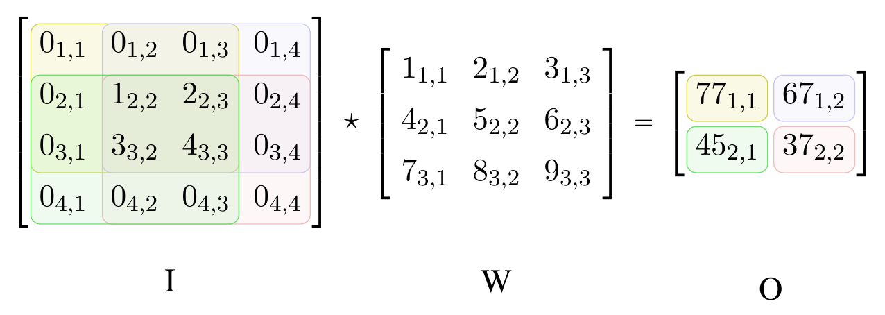
Figure 3. Cross-correlation between two matrices. Input matrix I has shape 4 × 4 and kernel matrix W has 3 × 3. The colored areas in I show the receptive field for each output in O. The matrix elements are numbered by their matrix indices.

Concrete example

Let us continue with another example in three dimensions. Our input I is a \(32 \times 32 \times 3\) tensor that represents an image with red, green and blue channels. Our filter W is a \(5 \times 5 \times 3\) tensor. We have one filter channel for each color channel. Now we convolve this filter by sliding it across the whole image. With that, we interact the color channels dimensions because we compute the dot product over three dimensions. The result is an activation map with dimensions \(28 \times 28\) because we can only place a \(5 \times 5\) filter only 28 times over a \(32 \times 32\) tensor. It is common to pad the input with a frame of zeros to control the first two dimension lengths of the output. For instance, a frame of zeros with thickness 2 maintains the first two dimension lengths of the input. Another option is to slide the filter with some stride to reduce the impact of the relations between close pixels on the filter weights. For instance, convolving the \(5 \times 5 \times 3\) filter over the \(32 \times 32 \times 3\) image with no padding and stride 2 results in an activation map of size \(16 \times 16 \times 3\) instead. Lastly, the CONV layer does not only use a single filter but a set of filters. E.g., with a set of seven filter, we obtain the same number of \(16 \times 16\) activation maps. We stack these activation maps along the third dimension of the resulting output tensor. Thus, we have transformed a \(32 \times 32 \times 3\) into a \(16 \times 16 \times 7\) stack of activation maps. Intuitively, each single filter has the capacity to detect specific local features in the input tensor that may be of importance to later layers. The weights in this filter tensor are parameters that we train with backpropagation.

General definition

A convolutional layer for images that are represented by a three dimensional input tensor is given by the following five components:

Input: a tensor \(I\) of size \(W_1 \times H_1 \times D_1\)
Hyperparameters: the number of filters \(K\), the filter’s width or height \(F\) (assuming both are equal), the stride \(S\) , and the amount of zero padding, \(P\).
Output: \(D_2\) different activation maps stored in a volume of size \(W_2 \times H_2 \times D_2\), where \(W_2= (W_1 - F+2P)/S+1\), \(H_2=(H_1-F+2P)S+1\), and \(D_2=K\).
Complexity: the number of parameters in each filter is \(F \times F \times D_1\). This gives a total of \(K \times (F \times F \times D_1) + K\) parameters for the whole layer. Note that the filter depth always equals the input depth. Moreover, the last \(K\) represents the bias terms that we add to the respective filter after each dot product computation with the data.
Operation: Each d-th slice of the output tensor (of size \(W_2 \times H2\)) is the result of computing the cross-correlation between the d-th filter over the input tensor with a stride of S and offsetting the result by d-th bias afterwards.

Cross-correlation slides each filter over the input with the same weights at every position. As a consequence, the size of the receptive field, i.e. the set of inputs that impact one output, is much smaller compared to fully-connected layers (cf. Figure 2. In particular, a convolutional layer is a special case of a fully connected layer, where many neurons have the same (re-arranged) set of weights and where most weights are set to zero except of a small neighborhood. Hence, the convolutional layer has much less parameters and is less prone to overfitting. To illustrate this point, let us consider the example of a \(128 \times 128 \times 3\) input image that is taken by a convolutional layer with 32 \(5 \times 5 \times 3\) filters, padding of 2 and a stride of 1. The output is a \(128 \times 128 \times 32\) volume consisting of \(524,288\) elements. We compute this volume with only \(32*5*5*3+32=2,432\) total parameters. In contrast, if this was a fully connect layer that computes every output element based on its own specific weights, we would use \(524,288 * (128 \times 128 \times 3) = 25,769,803,776\) parameters. This number is not only gigantic but it would also be difficult not to overfit the data even if we could store the parameters and compute the result.

Pooling layers

Another building block of CNNs are pooling layers. These layers are used to further reduce overfitting by downsampling the convolutions output with a fixed scheme and without any parameters. Specifically, these pooling operations are applied to each activation map separately and preserve the depth of the output volumes but not their height and width. As with cross-correlation, we slide the pooling filter over its input. However, we have to do this for each input channel separately because the pooling operation has no depth. A common setting is a \(2 \times 2\) filter with stride 2 where the filter represents a max operation over four numbers. This filter gives us an output tensor that is downsampled by \(2 \times 2\) along the first two dimensions.

Backward pass

The Jacobian of a convolution layer \(O = I \star W\) is given by \(I \star J^O\), where \(J^O\) is the Jacobian that contains the upstream gradients \(\delta^o\) with respect to the activation map parameters. This is illustrated by Figure 4. In comparison to the Jacobian for a fully-connected linear layer, the smaller, shared downstream gradient is only multiplied with the activations of its adjacent elements from the previous layer. The first derivatives of the pooling operations average and max are simple. The derivative of the average with respect to one element is 1 divided by the number of elements. The derivative of the max is the indicator function of maximum element’s index.

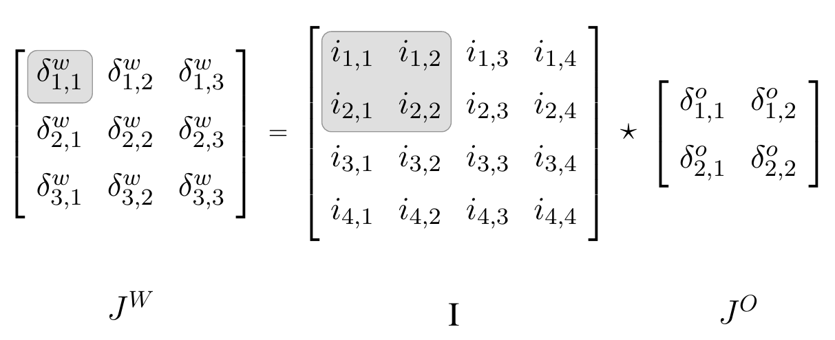
Figure 4. Backward pass through cross-correlation. The Jacobian J^W for the weight parameters of the cross-correlation O = I ⋆ W is given by the cross correlation between the Jacobian J^O that contains the downstream gradients δ^o with respect to the activation map parameters. The shaded area in I shows the elements that are used in the dot product with J^O to compute the shaded element in J^W.

CNN architectures

We build complete CNNs by stacking convolutional and pooling layers. A classical architecture is LeNet-5 for digit classification from black & white images of hand-written digits . A slightly simplified version has the form INPUT, [[CONV, POOL] \(\times\) 2], CONV, FC, FC, SOFTMAX. In this notation, INPUT stands for a tensor of a batch of images (\([100 \times 32 \times 32 \times 1]\) for a batch of 100 32 \(\times\) 32 black & white images), CONV denotes six, sixteen, and 120 \(5 \times 5\) filters with stride 1 and tanh activation, POOL denotes an average pooling layer with a 2 \(\times\) 2 filter and a stride of 2, and FC represents fully-connected layers. The first layer has tanh activations and the last layer calculates the softmax probabilities for ten different digits. The FC layers are used to extract features not only locally but globally and because this type of layer is cheaper after multiple rounds of downsampling. A receptive field of a (hidden) feature is the set if inputs that influence this feature. In a fully connected layer, the receptive field of every hidden feature is always the complete input vector or tensor. By stacking multiple convolutional layers, we can achieve the same receptive field with much less parameters. The outputs from higher layers have larger receptive fields and thus represent higher-level features. One example for these type of features could be far-reaching edges.

Lengthy network paths

In the last paragraph, we learned that classic CNN architectures are essentially a stack of functions. In Chapter 4, however, we saw that a sequence of function applications results in a long and linear backpropagation graph given by a multiplication sequence of partial derivatives. If a number of these partial derivatives are either very small or very large, their multiplicative effect can cause either too small or too large gradient updates during optimization. Especially layers with sigmoid activations (e.g. logistic, tanh) with derivatives that are flat or extremely steep for large parts of the domain are problematic. If parameters have once reached these parts, learning oftentimes stops for larger chunks of the network for two reasons. First, for these parameters, it requires a number of unusually large steps to leave these extreme areas. And second, other parameters with gradients that include multiplications with the extreme gradients are set to zero or infinity, too.

Skip connections

We can alleviate the problem by connecting earlier (or bottom) layers, \(h^{(i)}\), with later (or top) layers, \(h^{(i+k)}\), via the duplication operation followed by the "+" operator. With that, we open up a new path past the majority of the stacked functions. We call this type of link a skip connection. The effect is that, in the backward pass, \(l^{(i)}\) receives another downstream Jacobian \(J^{(i+k)}\cdot ... \cdot J^{(o)}\) that we add to the more complex Jacobian \(J^{(i+1)} \cdot J^{(i+2)} \cdot ... \cdot J^{(i+k)} \cdot... \cdot J^{(o)}\). Intuitively, the updates from the more complex Jacobian are used to learn the difference between the bottom layer and the top layer. As a result, we can learn a simple representation of the model without exposing the gradient to further multiplicative transformations and, in addition, we can learn another representation for more complex relations between the input features. An illustrative toy model similar to Figure 1 is \(C(\theta)= \tanh (\theta)^n\) where \(n \in \mathbb{N}^+\) represents the number of subsequent tanh operations. The model with skip connection is \(C_{res}(\theta)= C(\theta) + \theta\). We can observe the described technical aspects by comparing \(\partial C / \partial \theta\) with \(\partial C_{res} / \partial \theta\) and the respective computational graphs. An early implementation of this idea is Microsoft’s ResNet . This architecture uses skip connections that only skip one layer at a time. We will return to the problem of vanishing and exploding gradients from lenthy network parths in our discussion of recurrent neural networks.

Inductive bias

In the previous paragraph, we have seen how we can design neural network architectures to form sensible predictions on a domain-specific type of input data. We have also learned how to exploit the peculiar spatial relations in this data in order to save parameters and training time compared to fully-connected FNNs. The assumptions that we pose on the relations in the data in our architecture design is called the inductive bias. In summary, there are three inductive biases in the convolution layers of CNNs:

Translation equivariance: the convolution operation is translation eqiuivariant, i.e. \(f(x + dx) = f(x) + dx\) with input \(x\), change \(dx \in \mathbb{R}^n\) and \(f\) denotes the convolution operation. This means, if you apply a convolution operation to the original input and then apply the same operation to a translated version of the input, the resulting feature maps will have the same translation relationship. As a consequence, CNNs, which rely heavily on convolution operations, can learn to detect features in an image regardless of their spatial position. For example, a CNN trained to recognize cats will be able to detect a cat in different parts of an image because the learned features are translation equivariant. This reduces the need for manually designing position-specific features and allows CNNs to generalize well to various tasks involving spatial data. For other transformations than shifting, such as rotations and change in color, however, we need to train on additional augmented images.
Locality of features: the filter sizes are much smaller than the image because we assume that local relations between the pixels are more important than global relations.
Universality of feature extractors: we can reuse the same filter for all regions of the input because we assume that the hidden features which we extract are similarly important at each position.

In order to improve our results, we soften the inductive bias regarding the locality of features with two additional layers: at the beginning of the network, we include cheap pooling layers and towards the end we add fully connected layers.

Citation

In case you like this series, cite it with:

@misc{stenzel2023deeplearning,
  title   = "Deep Learning Series",
  author  = "Stenzel, Tobias",
  year    = "2023",
  url     = "https://www.tobiasstenzel.com/blog/2023/dl-overview/
}