7. Recurrent Neural Networks
🧱 The encoder-decoder RNN is quite useful for understanding the transformer.
Recurrent Neural Networks
Many tasks require input or output spaces that contain sequences. For example, in translation programs, words are often encoded as sequences of one-hot vectors. Each one-hot vector has a 1 at the position of an integer mapped to a word in a fixed vocabulary. A simple recurrent neural network (RNN) processes a sequence of vectors \(\{x_1, \dots, x_T\}\) using the recurrence formula:
\[\begin{align} h_t = f_\theta(h_{t-1}, x_t). \end{align}\]- \(f\) is a function (detailed below) that uses the same parameters \(\theta\) at every time step. This implies parameter sharing and introduces an inductive bias for modeling sequences.
- We can interpret the hidden vector \(h_t\) as a summary of all previous \(x\)-vectors.
- A common initialization is \(h_0 = \vec{0}\).
We can define \(f\) according to three criteria:
-
1. Input–Output Space
Depending on the task, we may want to handle “one-to-many,” “many-to-one,” or “many-to-many” mappings between the inputs and outputs. -
2. Order of Processing
The nature of the data may require:- Predicting \(y_t\) immediately after seeing \(x_t\).
- Predicting the entire output sequence \(\{y_1, \dots, y_T\}\) only after reading the full input sequence \(\{x_1, \dots, x_T\}\) in one shot.
- Predicting the output sequence bit by bit after reading the complete input in order to also include the output elements that where generated so far as information for the next prediction.
-
3. Handling Long Sequences
As sequences grow longer, we encounter drawbacks (e.g., vanishing/exploding gradients). We will address this point later in the section.
To illustrate how RNNs work, let us look at two specific examples. The first example is a vanilla RNN for predicting the next character in a text prompt. The second example is a token level encoder-decoder RNN for translation that can also work well with longer text. We will prepare this example with a longer explanation of the encoder-decoder architecture in general. Understanding this concept is crucial for understanding modern transformer based models. Finally, we look at the backward pass of the vanilla RNN to understand fundamental problems of RNNs in a deeper way.
Tokenization
The examples here use sequences of characters or words. However, in realistic applications text is mapped to a sequence of elements that are instances of a fixed vocabulary. This mapping is achieved by neural networks called tokenizers. Tokens can be anything from words, subword segments, or individual characters.
Vanilla Recurrent Neural Networks
Vanilla RNNs use a simple recurrence defined by:
\[\begin{align} h_t &= \phi \big ( W\begin{bmatrix} x_{t} \\ h_{t-1} \end{bmatrix} \big ). \label{eq:vanilla-rnn} \end{align}\]- We concatenate the current input \(x_t\) and the previous hidden state \(h_{t-1}\).
- We transform them linearly (by multiplying with \(W\)).
- We apply a non-linear activation \(\phi\).
In vector form, this is equivalent to:
\(\)\begin{align} h_t = \phi \big ( W_{xh}x_t + W_{hh}h_{t-1} \big ). \(\)\end{align}
- \(W_{xh}\) and \(W_{hh}\) are concatenated horizontally to form \(W\).
- If \(x_t \in \mathbb{R}^D\) and \(h_t \in \mathbb{R}^H\), then
\(\,W_{xh} \in \mathbb{R}^{H \times D}\)
\(\,W_{hh} \in \mathbb{R}^{H \times H}\)
\(\,W \in \mathbb{R}^{\,H \times (D+H)}.\)
Effectively, a vanilla RNN models the new hidden state \(h_t\) at each time step as a linear function of the previous hidden state \(h_{t-1}\), and the current input \(x_t\). Both inputs are passed through a non-linearity \(\phi\).
Example: Character-level Language Model
In a classification task—e.g., predicting the next character in a text prompt—one can apply a Softmax to a linear transformation of the hidden state at every time step:
\(\)\begin{align} o_t = W_{ho}\,h_t, \quad \hat{y}_t = \text{Softmax}(o_t), \end{align}\(\)
to predict the next character’s one-hot encoding. The linear transformation projects the hidden state into the alphabet space and the softmax function converts the real vector into the unit space. Then, we can use the character with the highest number as prediction. This is illustrated by Figure 5.
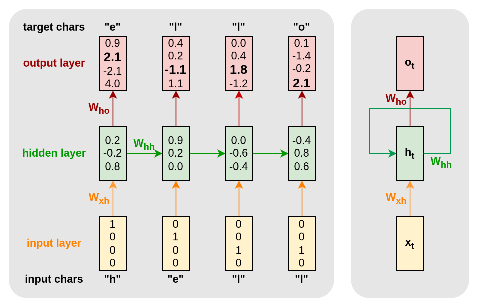
Figure 5. Vanilla RNN as character-level language model. The left side shows the unrolled RNN. The vocabulary has four characters and the training sequence is “hello”. Each letter is represented by a 1-hot encoding (yellow) and the RNN predicts the encodings of the next letter (green) at each time step. The RNN has a hidden state with three dimensions (red). The output has four dimensions. The dimensions are the logits for the next character. They are the softmax of a linear transformation of the hidden states. During supervised learning, the model will be trained to increase (decrease) the logits of the correct (false) characters. The right side shows the rolled-up RNN. The graph has a cycle that shows that the same hidden states are shared across time and that the architecture is the same for each step.
The Encoder–Decoder Architecture
An encoder–decoder model is build for applications that involve generating a sequence of potentially different length from another sequence. One such application is translation or question answering. In its most general case, the model transforms an input sequence \(\begin{align} X = \{x_1, x_2, \dots, x_{T_x}\} \end{align}\) into an output sequence \(\begin{align} \hat{Y} = \{\hat{y}_1, \hat{y}_2, \dots, \hat{y}_{T_y}\}. \end{align}\)
It is structured into two main components:
Encoder
Produces an internal representation \(R\) of \(X\). Formally:
\(\begin{align} R = \mathrm{Encoder}(X). \end{align}\)
- In some architectures, \(R\) is a single vector (often called a context).
- In others (e.g., with attention), \(R\) is a sequence of states \(\{h_1,\dots,h_{T_x}\}\).
- Or it may be multiple stacked layers of representations (e.g., in a Transformer).
Decoder
Generates each output element \(\hat{y}_t\) (for \(t=1,\dots,T_y\)) one at a time, with an autoregressive dependence on its own partial output and on the encoder representation \(R\). Concretely, we can think of the decoder in three submodules:
-
(a) Self-encoding of partial outputs
The decoder keeps a hidden state \(s_t\) that “remembers” what it has generated so far:
\[\begin{align} s_t^{(\mathrm{self})} = \mathrm{SelfEnc}\bigl(s_{t-1}^{(\mathrm{self})},\, \hat{y}_{t-1}\bigr). \end{align}\]This submodule accumulates the history \(\{\hat{y}_1, \dots, \hat{y}_{t-1}\}\) into \(s_t^{(\mathrm{self})}\).
-
(b) Cross-encoding (referencing the encoder)
The decoder also needs to incorporate the encoder’s representation \(R\). We denote this step by:
\(\begin{align}
s_t^{(\mathrm{cross})} = \mathrm{CrossEnc}\bigl(s_t^{(\mathrm{self})},\, R\bigr).
\end{align}\)
- In a simple setting, \(\mathrm{CrossEnc}\) might just copy or concatenate \(s_t^{(\mathrm{self})}\) with \(R\).
- In an attention-based setting, \(\mathrm{CrossEnc}\) might compute a new context \(\tilde{c}_t\) from \(\{h_1,\dots,h_{T_x}\}\) and combine that with \(s_t^{(\mathrm{self})}\).
- (c) Output module Finally, the decoder uses a function \(\mathrm{Output}\) to map \(s_t^{(\mathrm{cross})}\) to a distribution over possible next tokens: \(\begin{align} \hat{y}_t = \mathrm{Output}\bigl(s_t^{(\mathrm{cross})}\bigr). \end{align}\) Typically, \(\mathrm{Output}\) is a linear layer plus a softmax.
Altogether, the generic decoder step might look like:
\[\begin{align} \begin{aligned} s_t^{(\mathrm{self})} &= \mathrm{SelfEnc}\bigl(s_{t-1}^{(\mathrm{self})},\, \hat{y}_{t-1}\bigr),\\ s_t^{(\mathrm{cross})} &= \mathrm{CrossEnc}\bigl(s_t^{(\mathrm{self})},\, R\bigr),\\ \hat{y}_t &= \mathrm{Output}\bigl(s_t^{(\mathrm{cross})}\bigr). \end{aligned} \end{align}\]where \(\hat{y}_{t-1}\) is the decoder’s previous prediction.
In many actual implementations, submodules (a) and (b) may be fused into a single recurrent or feed-forward block. The above separation is conceptual, highlighting that the decoder is simultaneously encoding the partial outputs and referencing the encoder representation.
Dealing with Sequences of Different Lengths
To allow different input and output lengths, we introduce two special tokens:
- Start-of-sentence: \(\langle sos \rangle\)
- End-of-sentence: \(\langle eos \rangle\)
The encoder stops reading the input when it encounters \(\langle eos \rangle\). The decoder starts generating with \(\langle sos \rangle\) as \(y_1\) and stops when it generates \(\langle eos \rangle\).
Encoder-Decoder RNNs
We now specialize this generic view to an RNN-based encoder–decoder. We will (i) specify a fairly general RNN recurrence form, and then (ii) show how it can reduce to simple linear transformations with a standard nonlinearity.
General RNN Recurrence for Encoder and Decoder
-
Encoder RNN:
\(\begin{align} h_t = f_{\mathrm{enc}}(h_{t-1},\, x_t), \quad t=1,\dots,T_x, \end{align}\) with some initialization \(h_0\). We take the final state \(h_{T_x}\) as \(\begin{align} R = h_{T_x}, \end{align}\) a single “context vector.” -
Decoder RNN: merges self-encoding and cross-encoding into a single update: \(\begin{align} s_t = f_{\mathrm{dec}}\bigl(s_{t-1},\, \hat{y}_{t-1},\, R\bigr), \quad t=1,\dots,T_y, \end{align}\) and then \(\begin{align} \hat{y}_t = \mathrm{Output}\bigl(s_t\bigr). \end{align}\) This single function \(f_{\mathrm{dec}}\) effectively does:
- Encode the partial outputs via \(\hat{y}_{t-1}\) and \(s_{t-1}\).
- Cross-encode the encoder’s context \(R\).
Vanilla Encoder-Decoder RNN
In the simplest “vanilla” RNN, the encoder might be:
\(\begin{align} h_t = \phi\Bigl( W_{\mathrm{enc}}^{(hh)}\,h_{t-1} \;+\; W_{\mathrm{enc}}^{(xh)}\,x_t \Bigr), \end{align}\) where \(\phi(\cdot)\) is a nonlinearity (e.g. \(\tanh\)). Then we set
\[\begin{align} R = h_{T_x}. \end{align}\]For the decoder, we can define:
-
Initialization: \(\begin{align} s_0 = R = h_{T_x}. \end{align}\)
-
Recurrent update: \(\begin{align} s_t = \phi\Bigl( W_{\mathrm{dec}}^{(ss)}\,s_{t-1} \;+\; W_{\mathrm{dec}}^{(ys)}\,\hat{y}_{t-1} \;+\; W_{\mathrm{dec}}^{(cs)}\,R \Bigr). \end{align}\) This merges the partial output (via \(\hat{y}_{t-1}\)) with the context \(R\).
-
Output module: \(\begin{align} \hat{y}_t = \mathrm{Softmax}\Bigl( W_{\mathrm{dec}}^{(so)}\,s_t \Bigr). \end{align}\)
In this concrete instantiation, submodules (a) and (b) from the generic description appear in a single formula for \(s_t\). The output module is simply a linear (via \(W_{\mathrm{dec}}^{(so)}\)) plus softmax layer.
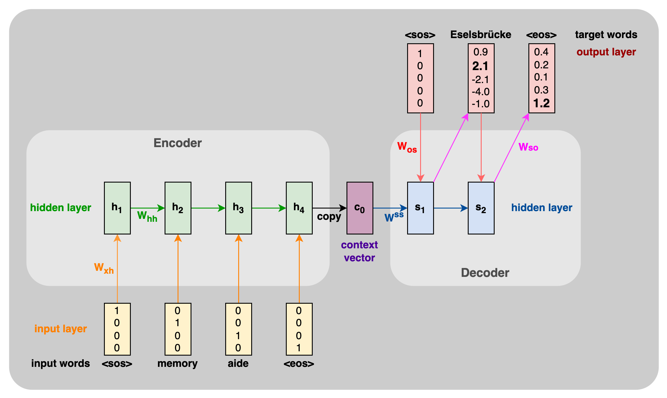
Figure 6. Encoder-Decoder RNN as word-level language model. The input
language has two and the output language has three words. Every word,
the start and the end of a sentence are represented by a one-hot
encoding (yellow) and the RNN predicts the encodings of the translation
of the input sentence. The encoder RNN has a hidden state (green) that
is updated by one word step-by-step to produce the final context vector
(purple). The decoder RNN takes linear functions of the final encoding
and the start embedding to compute the hidden states for the next output
embedding (blue). The one-hot encoding of the output words (red) are a
softmax of a linar function of these hidden states. The decoder RNN
iterates the prediction until it returns the end token. With this
architecture, we can predict sequences of arbitrary length using the
embedded information of a whole input sequence.
The simplicity of the RNN’s formulation has two drawbacks.
- The connections between inputs and hidden states through linear layers and element-wise non-linearities is not flexible enough for some tasks.
- The recurrent graph structure leads to problematic dynamics during the backward pass.
The Exploding and Vanishing Gradient Problem
We now explore the second problem—vanishing and exploding gradients—more formally. Consider the vanilla RNN’s loss with respect to the weight matrix in Equation \(\ref{eq:vanilla-rnn}\). Its derivative can be written as:
\(\) \begin{align} \frac{\partial L}{\partial W} = \sum_{t=1}^T \sum_{k=1}^{t+1} \frac{\partial L_{t+1}}{\partial o_{t+1}} \frac{\partial o_{t+1}}{\partial h_{t+1}} \frac{\partial h_{t+1}}{\partial h_{k}} \frac{\partial h_{k}}{\partial W}. \label{eq:rnn-derivative} \end{align} \(\)
A key factor here is the derivative of the hidden state at time \(t+1\) with respect to a past hidden state \(h_k\). From the chain rule, it follows a recursive product:
\(\) \begin{align} \label{eq:rnn-derivative-recursion} \frac{\partial h_{t+1}}{\partial h_k} = \prod_{j=k}^t \frac{\partial h_{j+1}}{\partial h_j} = \frac{\partial h_{t+1}}{\partial h_t} \cdot \frac{\partial h_t}{\partial h_{t-1}} \cdots \frac{\partial h_{k+1}}{\partial h_k} = \prod_{j=k}^t \mathrm{diag} \bigl( W_{hh} \,\phi’\bigl(W[x_{j+1} ;\,h_j]\bigr) \bigr). \end{align} \(\)
In essence, \(\frac{\partial h_{t+1}}{\partial h_k}\) is the product of Jacobians from time \(t\) down to \(k\). Because an RNN processes sequences, this product can become very large if \((t-k)\) is large (i.e., if the sequence is long).
Vanishing and Exploding Effects
To see why gradients may vanish or explode, assume for simplicity that each local Jacobian \(\tfrac{\partial h_{t+1}}{\partial h_t}\) is constant over time. Let us denote this constant Jacobian by \(J\). Suppose we decompose \(J\) via its eigendecomposition, yielding eigenvalues \(\lambda_1, \lambda_2, \dots, \lambda_n\) and corresponding eigenvectors \(v_1, v_2, \dots, v_n\), with
\(\) \begin{align} |\lambda_1| \geq |\lambda_2| \geq \cdots \geq |\lambda_n|. \end{align} \(\)
- Exploding Gradients: If \(\lvert\lambda_1\rvert > 1\), then repeated multiplications by \(J\) cause gradients to grow exponentially, leading to exploding gradients.
- Vanishing Gradients: Conversely, if \(\lvert\lambda_1\rvert < 1\), the gradient norms shrink exponentially as they propagate back through time, eventually becoming negligibly small (vanishing).
In practice, vanishing gradients are especially common when activation derivatives \(\phi'\) stay below 1 in magnitude (as with sigmoid or tanh). As a result, the earliest hidden states in the sequence receive almost no gradient information, hurting the model’s ability to capture long-range dependencies and effectively limiting its “long-term memory.”
Mitigation Strategies
Various methods aim to alleviate exploding or vanishing gradients. Examples include:
- Regularization (e.g., gradient clipping)
- Careful weight initialization
- ReLU activations
- Gated RNNs (LSTM or GRU), which introduce gating mechanisms akin to more sophisticated skip connections from Chapter 5
- Transformer architectures, which rely on attention instead of purely recurrent connections and thus suffer less from vanishing gradients while providing more expressive long-range interactions.
Today, the most widely used approach in many sequence tasks is the transformer, which not only avoids many vanishing-gradient issues but also offers more flexible and powerful modeling of contextual information.
Citation
In case you like this series, cite it with:
@misc{stenzel2023deeplearning,
  title   = "Deep Learning Series",
  author  = "Stenzel, Tobias",
  year    = "2023",
  url     = "https://www.tobiasstenzel.com/blog/2023/dl-overview/
}