5. Feedforward Neural Networks
Feedforward Neural Networks
In the last sections we learned that we can compute any differentiable loss function between an arbitrary differentiable function \(f\) that takes input \(x\) and outputs predictions \(\hat{y}\) and the data \((x,y)\), and optimize the model \(f\) with respect to its parameters \(\theta\) with stochastic gradient descent. In this section, we look at how to construct \(f\) as a neural network.
Vanilla Neural Networks
In the two examples from Chapter 2, neural network regression and
neural network classification, we have already discovered one main idea
of vanilla neural networks: combining matrix multiplications and
element-wise non-linearities. The other idea is that we can repeat, or
layer, these two transformations multiple times. For instance,
abstracting from the concrete structure of the input and output data, we
would write a neural network with two fully connected layers as
\(f(x)=W_1 \phi (W_1 x)\), where \(\phi\) represents an an element-wise
non-linearity like tanh and \(W_1\), \(W_2\) are matrices that interact,
scale, and shift the inputs. A 3-layer neural networks would be
implemented as \(f(x)=W_3 \phi (W_1 \phi (W_1 x))\), and so forth. The
outputs from the intermediate functions are called hidden layers, and
one output a hidden unit. We can think of hidden units as feature
abstractions from the previous layer, or latent features for the next
layer. During training, the neural network learns which feature
abstractions are useful to the next layer. A network is called deep if
it has more than one hidden layer. Common choices for non-linearity
\(\phi\) are tanh, the rectified linear unit (ReLU) \(\max(0,x)\), and the
logistic function \(1/(1+e^{-x})\). Usually, we add an additional element
\(x_0 = 1\) to the input vector. The corresponding weight, or bias,
\(b:=w_0\) shifts the output. The choice of the last layer depends on the
type of output data \(y\). For instance, we could select the logistic
function for binary classification, the softmax function for multi-class
classification, and a linear layer to predict natural numbers. Similar
to our toy example in Figure 1
reference=”fig:toy_graph”}, we can depict a vanilla neural network as a
directed acyclical graph and compute its gradient via backpropagation in
a supervised learning setting. Figure
2 depicts a two-layer example
architecture for a binary classification task. Note the similarity
between this network and the second example from Chapter 2. Figure
2 clarifies how we aggregate dot
product operations on the neuron level to matrix operations on the layer
level. In the last decade, the neural network approach has led to
state-of-the-art results in areas with large amounts of high-quality
data such as computer vision, natural language processing, speech
recognition and others. A theoretical reason for this success is that
neural networks can achieve universal approximation. This means that
they can approximate any continuous function, either via sufficient
depth (number of layers; e.g.
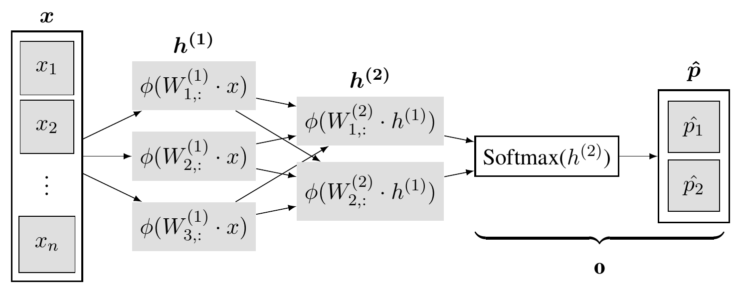
Figure 2. Vanilla neural network with two fully-connected hidden layers for binary classification. The first hidden layer, \(h^{(1)}\), is composed of three neurons. Each neuron takes the input vector \(x\) and computes the dot product with its weight vector from its respective column of the layer’s weight matrix \(W^{(1)}\). Moreover, \(h^{(1)}\) introduces non-linearity via an elementwise non-linear operation \(\phi\). The second layer, \(h^{(2)}\), repeats the same process with the previous hidden layer as its input but reduces the number of hidden features. The output layer $o$ has the same size as the last hidden layer and computes the Softmax probabilities for classes one and two.
Backward pass
To improve our understanding about backpropagation of neural networks, we look at the partial derivatives of typical layers. Note that we usually consider the derivatives with respect to the loss instead of the cost function because the regularization terms are not complex and simply add up to the more complicated loss derivative at the end of each update computation.
-
ReLU: the derivative of the element-wise ReLU is given by \(\frac{\partial ReLU}{\partial z} = 0\) if \(x \leq\) 0 and 1 if x \(>\) 0. As a consequence, we propagate only the gradient for the neurons with positive activations back to the previous layer.
-
Linear layer: Let \(z = W x\) be a linear layer with one input channel and \(n\) elements, \(x \in \mathbb{R}^{n \times 1}\), with \(W \in \mathbb{R}^{m \times n}\) and let \(z, \delta := \frac{\partial L}{\partial z} \in \mathbb{R}^{m \times 1}\). Then \(\frac{\partial L}{\partial W} = \frac{\partial L}{\partial z} \frac{\partial z}{\partial W} = \delta x^T\). The same result, \(\delta X^T\), holds for linear layers with \(k\) features or input channels, i.e. with \(X \in \mathbb{R}^{n \times k}\) and \(Z, \delta \in \mathbb{R}^{m \times k}\). Hence, each input receives the input-specic respective weighted sum of the upstream gradient of all neurons from the next layer.
-
Softmax: Let \(\hat{p}=\text{softmax}(z)\) denote the softmax probabiltities with \(\hat{p}, z \in \mathbb{R}^{n \times m}\) and let \(L(\hat{p},y)\) with \(y \in \mathbb{R}^{n \times 1}\) be the scalar cross-entropy loss. We get \(\frac{\partial L}{\partial z} = \frac{1}{n}(\hat{p} - y \otimes \vec{1}^m )\), where \(\otimes\) denotes the outer product between two vectors. If we add another logit layer \(l\in \mathbb{R}^{n \times m}\) below the softmax, we obtain the following simple result:
- Intuitively, for each example \(i \in 1,...,n\), the gradients for each parameter that flow from each predicted probability is increased by the amount that the predicted probability differs from the actual label (times \(1/n\)). Therefore, gradient descent in particular updates parameters \(\theta\) towards the direction of the gradients from the bad predictions.
Citation
In case you like this series, cite it with:
@misc{stenzel2023deeplearning,
  title   = "Deep Learning Series",
  author  = "Stenzel, Tobias",
  year    = "2023",
  url     = "https://www.tobiasstenzel.com/blog/2023/dl-overview/
}