3. Optimization
Optimization
In the previous section we formalized supervised learning of a predictive model as solving the optimization problem \(\theta^* = \arg \min_{\theta \in \Theta} C(\theta)\), where \(\theta\) denotes the model parameters and cost function \(C\) represents the average loss of all examples plus a regularization penalty. In realistic settings, there is no closed form solution to this problem. Therefore, we have to rely on schemes that iteratively proposes new parameters given the previous choice or the initial guess. We want to choose a method that proposes new candidates with a high likelihood of reducing the loss compared to the current parameters, so we can replace them.
First order methods
In practice, a neural network is a composition of many small functions that are easy to differentiate. Therefore, we can compute the gradient \(\nabla_\theta C\) from our network via the backpropagation technique. We will discuss this method in detail in the next section. The gradient of our cost function is a vector of first-order partial derivatives. It contains the direction of its fastest increase and its magnitude is the rate of increase in that direction. The gradient at a minimum of the loss function equals zero. Therefore, we can use the negative gradient as search direction for selecting the next proposal \(\theta_{i+1}\) from current candidate \(\theta_i\). This is the basic idea of the gradient descent algorithm. The method alternates between two steps: 1.) Compute the gradient \(\nabla_\theta C(\theta)\). 2.) Update \(\theta\) by subtracting a small multiple of the gradient. Many applications use very large datasets. For instance, the number of training images in ImageNet is about 1 million. Therefore, it is handy to approximate the loss gradient from a small minibatch of examples (e.g. 100). With that, we can update \(\theta\) many times for every epoch. An epoch is one iteration over the complete training set. In practice, a large number of approximate updates works better than a small number of exact updates. This algorithm is called Stochastic Gradient Descent (SGD). It is summarized in Algorithm 1.
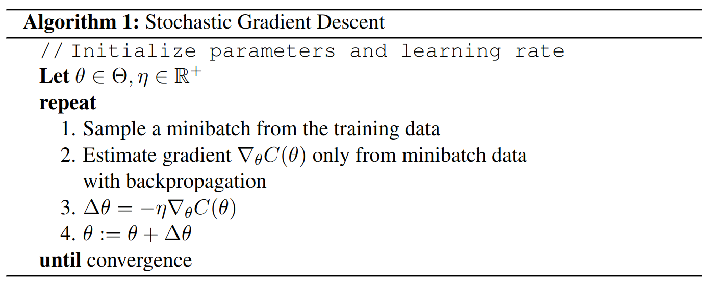
A crucial parameter for gradient descent algorithms is the learning rate, or step size, \(\eta\). If we set it too small, the optimization requires too many steps. If we set it too large, the algorithm may not converge or even diverge. As an illustration, consider the following toy example with convex objective function: Let \(f=x^2\) with gradient \(\frac{df}{dx}=2x\) and initial parameter value \(x = 1\). With \(\eta<1\) the algorithm finds \(x^*=0\). However, with \(\eta=1\), it oscillates between \(x=-1\) and \(x=1\), and with \(\eta>1\) it diverges to \(x=\infty\). Generally, finding a useful learning rate depends on the objective function.
Advanced first order methods
Oftentimes, we can achieve faster
convergence speed with modified formulations of the update direction
\(\Delta \theta\) from Step 3 in Algorithm 1. The
two main ideas are to use weighted moving averages of all gradients so
far and to compute parameter-specific learning rates. Common variants
are Momentum
Hyperparamter optimization
In the discussion of supervised learning
and optimization, we encountered many configurations that we did not
specify. Examples are the number of hidden units \(H\) in our neural
network, the regularization strength \(\lambda\), or the learning rate
\(\eta\) in gradient descent. These parameters either change the
composition of the model parameters \(\lambda\) or impact their selection
during training. Therefore, they have to be set before a model is
trained. To this end, we have to select our hyperparameter space
\(\mathcal{H}\). Due to restrictions of time and computational power, this
choice is often based on experiences with similar models from previous
research. Principled approaches range from model-free methods like
random search to global optimization frameworks like Bayesian
optimization. Model-free methods are simple and do not use the
evaluation history whereas global optimization techniques additionally
consider the uncertain trade-off between exploring new values and
exploiting good values that have already been found. I recommend the
textbook chapter by
Citation
In case you like this series, cite it with:
@misc{stenzel2023deeplearning,
  title   = "Deep Learning Series",
  author  = "Stenzel, Tobias",
  year    = "2023",
  url     = "https://www.tobiasstenzel.com/blog/2023/dl-overview/
}